
Recommandé
Contenu connexe
Tendances
Similaire à Lec60
Dernier
Dernier (20)
Lec60
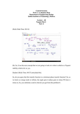
- 1. Control Systems Prof. C. S. Shankar Ram Department of Engineering Design Indian Institute of Technology, Madras Lecture – 60 Nyquist Plot 2 Part -2 (Refer Slide Time: 00:14) Ok. So, if not the next concept that we are going to look at is what is called as a Nyquist stability criteria ok; so, yes. Student: (Refer Time: 00:37) articulated this. So, do you agree that this transfer function is a minimum phase transfer function? So, as we know as omega tends to infinity, the angle goes to phase goes to minus 90 times n minus m. So, you substitute n and m what do you get from this problem 0.
- 2. (Refer Slide Time: 00:57) And then you go to the Nyquist plot what where is the transfer function as omega tends to infinity? Student: 1 Plus 1. You draw a vector from 0 to 1, what is the angle made with a vector, 0 degrees all right. (Refer Slide Time: 01:10)
- 3. So, I am just using the Nyquist plot to just if you draw the bode plot, you will once again observe the same thing. I am just interpreting it from the Nyquist plot that is all I am doing right yeah ok. So, one important application of the Nyquist plot is what is what to say to figure out these stability of the closed loop system right. So, so if you recall our notion our block diagram, you know like of the closed loop system that we have been looking at is that like the forward path transfer function was a G of s if you recall ok. So, this is E of s right, and this is Y of s. And the feedback path transfer function is going to be H of s. And this is going to close the loop let us say we have negative feedback let me call the signal as W of s right. So, this is the block diagram we have. ah What is a closed loop transfer function? Recall that Y of s divided by R of s is going to be equal to G of s divided by 1 plus G of s H of s right. So, this is the closed loop transfer function ok. So, now how do we once again like determine whether the closed loop system is stable say I am only asking the same questions again right, we are revisiting the same points right. How do we check out the stability of the closed loop system, we look at the closed loop characteristic equation, so the roots of this equation or the closed loop pole right. So, this is the closed loop characteristic equation ok. And you immediately see that the closed loop characteristic polynomial is going to be equal to 1 plus G of s times H of s that is what we have right that is the closed loop characteristic polynomial right. So, let G of s times H of s be n o s divided by d o s. So, the I am using the subscript o to indicate that that is the open loop transfer functions numerator and denominator. See, in general rewrite any transfer function as a ratio of two polynomials in s numerator polynomial n of s and denominator polynomial d of s right that is what we have been doing right. So, I am just saying it as n o of s divided by d o of s right, so that is what we have ok. So, this implies that 1 plus G of s H of s is going to be equal to 1 plus n o of s divided by d o of s which is nothing but d o of s divided by n o of s divided by d o of s. So, we will see why I am doing all these things, so because I want to set some terminology in order before we go in go further right.
- 4. (Refer Slide Time: 04:49) So, this immediately tells me that you can immediately see that the poles of 1 plus G of s H of s are what are they. So, if you consider the closed loop characteristic polynomial 1 plus G of s H of s right, that is going to be a ratio of two polynomials in s, is it not, it is also a ratio of two polynomials in s. What is the denominator polynomial. Student: (Refer Time: 05:28). d o of s. What are the roots of d o of s called as? Student: (Refer Time: 05:33). Poles of what? Student: (Refer Time: 05:35). Open loop poles. Please remember that because d o of s is the what to say the denominator polynomial of the open loop transfer function. So, immediately you see that the poles of 1 plus G of s H of s are the open loop poles. Are these known in general? By and large they are under our control right because what do the open loop poles constitute, they constitute the what to say the planned poles controller transfer function pole and the feedback path transfer function pole. So, in general at least we will be able to tune them even if the controller contribute some open loop poles, we will be able to tune them. So, we know what these poles are right
- 5. yeah. So, what can you say about the zeros of 1 plus G of s H of s. What are the zeros of the zeros of the polynomial closed loop characteristic polynomial 1 plus G of s H of s called as, we already discuss this I am just recapping. Student: (Refer Time: 07:00) closed loop poles. Closed loop poles that is it right so yeah. So, I am recapping this terminology once again because we are going to mix poles and zeros right, but I want us to be very clear I am considering the polynomial 1 plus G of s H of s which is a ratio of two polynomials. It so happens that the denominator polynomial of 1 plus G of s H of s is the same as the denominator polynomial of the open loop transfer function. So, the poles of 1 plus G of s H of s are nothing but the open loop poles. The zeros of 1 plus G of s H of s are the closed loop poles. This is one which is of importance for us right, because we are when we designed the closed loop system, we are worried about the closed loop poles, open poles are already given to us right. We are worried about what are the closed loop poles. In other words what are the zeros of one plus G of s H of s, is it clear. Now, please remember this what to say terminology, we are going to pose a question. Yes, please. Student: (Refer Time: 08:04) Why, why and why should they be closed loop zeros, no, but 1 plus d of s in the denominator of the closed loop transfer function right. Is not it? I am extracting that is why I am doing it carefully step by step. So, please go back and of course, very natural question because I am extracting the denominator then I am writing the denominator of the closed loop transfer function as a ratio of one another numerator denominator then I am processing it right, so that is why I am doing it step by step. But from here onwards, I will just use this terminology that is why we came to this all right. Now, the question that we are asking ourselves, we are going to ask ourselves; and the question the answer to which would be provided by the Nyquist stability criteria is the following.
- 6. (Refer Slide Time: 10:09) Given the open loop transfer function g of s times H of s that means, we know the open loop poles can we comment about the stability of the closed loop system using the Nyquist plot of the open loop transfer function G of s H of s. This is a question we are going to ask ourselves ok. So, let me repeat the question. So, let us read the question that is you are given the open loop transfer function G of s H of s right by enlarge it is known right. So, we know the open loop poles right. So, open loop poles are nothing but the poles of 1 plus G of s H of s. Please remember that right, so as we seen the green box right. So, open loop poles are nothing but poles of one plus G of s H of s we know them right. Given the open loop transfer function can we then use the Nyquist plot of the open loop transfer function G of s H of s to comment about this close loop stability that is what we are asking ourselves. And of course, the answer is yes that is why we have the Nyquist stability criteria. So, but the general result on which this stability criteria rests on is what is called as the mapping theorem in complex algebra there is something called as a mapping theorem. Once again I am not going to prove any of this we are just going to use them. The mapping theorem reads to of course, this is the answer of course, the answer is yes how you know like them, we will visit what is called as a mapping theorem. And the mapping theorem leads to what is called as a Nyquist stability criterion. So, this is what I have
- 7. typed in that handout ok. So, what I want you to do is that now I want you to read through the handout, if you are not already done. So, if you go to the course website below root locus construction, I have I have uploaded another file called Nyquist stability criteria. I hope you are able to access that file right. So, in that I have clearly typed what is the mapping theorem and how it is applied to the Nyquist stability criteria. Kindly go through the document and come to the next class we would discuss the same all right in the next class. But I am going to leave you with another question please think through these questions. Let us say let the plot of G of j omega H of j omega that is the open loop sinusoidal transfer function. So, G of s H of s you substitute s equals j omega you get the open loop sinusoidal transfer function. And let this be given for omega belonging to 0 to infinity ok, so that is what we have plotted as a Nyquist plot right. You give me any transfer function that is a Nyquist plot. (Refer Slide Time: 13:46) See for example let us say just for a sake of example. Let us say the transfer function s plus one divided by s plus 10 was the open loop transfer function let us say right. We have plotted the Nyquist plot of that as omega varies from 0 to infinity. So, till now we have been looking at omega as a physical parameter right, where you know like it is associated with frequency and it can take only positive values. But when
- 8. we go to this mapping theorem and Nyquist stability criteria, we are going to look at omega as a real parameter and it can take values from minus infinity to plus infinity ok. We will learn that in the next class. So, if that is the case, how can one obtain the plot of G of j omega H of j omega for omega between minus infinity to 0. So, the Nyquist plot you now like by definition it is a plot of any transfer function by substituting s equals 0 omega and you plot from omega going from 0 to infinity that is the definition. But let us say instead let us now look at omega as a parameter or rather than associating the meaning of frequency. So, let us say I substitute s equals j omega, omega is now a parameter and that parameter can vary from let us say minus infinity to plus infinity. So, I am given already the Nyquist plot of the transfer function when omega varies from 0 to infinity. How can I get the Nyquist plot of the same transfer function, when it when I go from minus infinity to 0 ok. Please try this one out for all the transfer functions that we are plotted till now, and then like figure things out right what happens. So, let me do for one example and then of course, I am I am going to let you extrapolate ok. So, I am just going to do one example and then we will see. See, for example, we did 1 by s all right, G of s was 1 by s. So, this means that it is essentially minus j by sorry G of j omega was 1 by j omega right. So, this is minus j by omega. So, now if I have omega to be non positive that is it comes from minus infinity to 0, what do you think will happen, let us plot. So, what was the Nyquist plot when it came from 0 to infinity, as it reached infinity where it would go? Student: (Refer Time: 16:49). We did it yesterday right. The Nyquist plot was the negative real imaginary axis this was omega tending to 0; this is omega tending to infinity. Let us say it is the other way around, what will happen? When it goes from minus infinity to 0 what do you think will happen, what is the value as it tends to minus infinity anyway it will be 0. And for as it goes to 0, it will blow off to plus infinity because it is coming from the negative side. So, what will happen is then it will also start from this as it goes from minus ready and then it will go to plus this is omega tending to 0 minus. So, I am just going to put a 0 plus
- 9. and 0 minus just to indicate that from which side am I coming to 0 all right. 0 plus means I am coming going to 0 from the right ok; 0 minus means I am coming to 0 from the left from the negative real axis right negative side. But of course, this is a very special example, so you will see that you will have a what to say radius of a sorry semicircle of infinite radius as your Nyquist plot, but this is a very special example. I am just giving you one example for to show you how to do that right. So, kindly plot the first order factor that we looked at and then tell me what you will get when you have omega as a parameter which varies from minus infinity to plus infinity so that is something which I am going to leave it to us as homework fine. So, when we meet in the next class you know like we will look at the mapping theorem and then like we will also discuss the Nyquist stability criterion.