interpolation lagrange

1. Jim Lambers
MAT 772
Fall Semester 2010-11
Lecture 5 Notes
These notes correspond to Sections 6.2 and 6.3 in the text.
Lagrange Interpolation
Calculus provides many tools that can be used to understand the behavior of functions, but in most
cases it is necessary for these functions to be continuous or differentiable. This presents a problem
in most “real” applications, in which functions are used to model relationships between quantities,
but our only knowledge of these functions consists of a set of discrete data points, where the data
is obtained from measurements. Therefore, we need to be able to construct continuous functions
based on discrete data.
The problem of constructing such a continuous function is called data fitting. In this lecture,
we discuss a special case of data fitting known as interpolation, in which the goal is to find a
linear combination of 𝑛 known functions to fit a set of data that imposes 𝑛 constraints, thus
guaranteeing a unique solution that fits the data exactly, rather than approximately. The broader
term “constraints” is used, rather than simply “data points”, since the description of the data may
include additional information such as rates of change or requirements that the fitting function
have a certain number of continuous derivatives.
When it comes to the study of functions using calculus, polynomials are particularly simple to
work with. Therefore, in this course we will focus on the problem of constructing a polynomial
that, in some sense, fits given data. We first discuss some algorithms for computing the unique
polynomial 𝑝𝑛(𝑥) of degree 𝑛 that satisfies 𝑝𝑛(𝑥𝑖) = 𝑦𝑖, 𝑖 = 0, . . . , 𝑛, where the points (𝑥𝑖, 𝑦𝑖) are
given. The points 𝑥0, 𝑥1, . . . , 𝑥𝑛 are called interpolation points. The polynomial 𝑝𝑛(𝑥) is called the
interpolating polynomial of the data (𝑥0, 𝑦0), (𝑥1, 𝑦1), . . ., (𝑥𝑛, 𝑦𝑛). At first, we will assume that the
interpolation points are all distinct; this assumption will be relaxed in a later lecture.
If the interpolation points 𝑥0, . . . , 𝑥𝑛 are distinct, then the process of finding a polynomial that
passes through the points (𝑥𝑖, 𝑦𝑖), 𝑖 = 0, . . . , 𝑛, is equivalent to solving a system of linear equations
𝐴x = b that has a unique solution. However, different algorithms for computing the interpolating
polynomial use a different 𝐴, since they each use a different basis for the space of polynomials of
degree ≤ 𝑛.
The most straightforward method of computing the interpolation polynomial is to form the
system 𝐴x = b where 𝑏𝑖 = 𝑦𝑖, 𝑖 = 0, . . . , 𝑛, and the entries of 𝐴 are defined by 𝑎𝑖𝑗 = 𝑝𝑗(𝑥𝑖),
𝑖, 𝑗 = 0, . . . , 𝑛, where 𝑥0, 𝑥1, . . . , 𝑥𝑛 are the points at which the data 𝑦0, 𝑦1, . . . , 𝑦𝑛 are obtained, and
𝑝𝑗(𝑥) = 𝑥𝑗, 𝑗 = 0, 1, . . . , 𝑛. The basis {1, 𝑥, . . . , 𝑥𝑛} of the space of polynomials of degree 𝑛 + 1
is called the monomial basis, and the corresponding matrix 𝐴 is called the Vandermonde matrix
1

2. for the points 𝑥0, 𝑥1, . . . , 𝑥𝑛. Unfortunately, this matrix can be ill-conditioned, especially when
interpolation points are close together.
In Lagrange interpolation, the matrix 𝐴 is simply the identity matrix, by virtue of the fact that
the interpolating polynomial is written in the form
𝑝𝑛(𝑥) =
𝑛∑
𝑗=0
𝑦𝑗ℒ𝑛,𝑗(𝑥),
where the polynomials {ℒ𝑛,𝑗}𝑛
𝑗=0 have the property that
ℒ𝑛,𝑗(𝑥𝑖) =
{
1 if 𝑖 = 𝑗
0 if 𝑖 ∕= 𝑗
.
The polynomials {ℒ𝑛,𝑗}, 𝑗 = 0, . . . , 𝑛, are called the Lagrange polynomials for the interpolation
points 𝑥0, 𝑥1, . . ., 𝑥𝑛. They are defined by
ℒ𝑛,𝑗(𝑥) =
𝑛∏
𝑘=0,𝑘∕=𝑗
𝑥 − 𝑥𝑘
𝑥𝑗 − 𝑥𝑘
.
As the following result indicates, the problem of polynomial interpolation can be solved using
Lagrange polynomials.
Theorem Let 𝑥0, 𝑥1, . . . , 𝑥𝑛 be 𝑛 + 1 distinct numbers, and let 𝑓(𝑥) be a function defined on a
domain containing these numbers. Then the polynomial defined by
𝑝𝑛(𝑥) =
𝑛∑
𝑗=0
𝑓(𝑥𝑗)ℒ𝑛,𝑗
is the unique polynomial of degree 𝑛 that satisfies
𝑝𝑛(𝑥𝑗) = 𝑓(𝑥𝑗), 𝑗 = 0, 1, . . . , 𝑛.
The polynomial 𝑝𝑛(𝑥) is called the interpolating polynomial of 𝑓(𝑥). We say that 𝑝𝑛(𝑥) interpolates
𝑓(𝑥) at the points 𝑥0, 𝑥1, . . . , 𝑥𝑛.
Example We will use Lagrange interpolation to find the unique polynomial 𝑝3(𝑥), of degree 3 or
less, that agrees with the following data:
𝑖 𝑥𝑖 𝑦𝑖
0 −1 3
1 0 −4
2 1 5
3 2 −6
2

3. In other words, we must have 𝑝3(−1) = 3, 𝑝3(0) = −4, 𝑝3(1) = 5, and 𝑝3(2) = −6.
First, we construct the Lagrange polynomials {ℒ3,𝑗(𝑥)}3
𝑗=0, using the formula
ℒ𝑛,𝑗(𝑥) =
3∏
𝑖=0,𝑖∕=𝑗
(𝑥 − 𝑥𝑖)
(𝑥𝑗 − 𝑥𝑖)
.
This yields
ℒ3,0(𝑥) =
(𝑥 − 𝑥1)(𝑥 − 𝑥2)(𝑥 − 𝑥3)
(𝑥0 − 𝑥1)(𝑥0 − 𝑥2)(𝑥0 − 𝑥3)
=
(𝑥 − 0)(𝑥 − 1)(𝑥 − 2)
(−1 − 0)(−1 − 1)(−1 − 2)
=
𝑥(𝑥2 − 3𝑥 + 2)
(−1)(−2)(−3)
= −
1
6
(𝑥3
− 3𝑥2
+ 2𝑥)
ℒ3,1(𝑥) =
(𝑥 − 𝑥0)(𝑥 − 𝑥2)(𝑥 − 𝑥3)
(𝑥1 − 𝑥0)(𝑥1 − 𝑥2)(𝑥1 − 𝑥3)
=
(𝑥 + 1)(𝑥 − 1)(𝑥 − 2)
(0 + 1)(0 − 1)(0 − 2)
=
(𝑥2 − 1)(𝑥 − 2)
(1)(−1)(−2)
=
1
2
(𝑥3
− 2𝑥2
− 𝑥 + 2)
ℒ3,2(𝑥) =
(𝑥 − 𝑥0)(𝑥 − 𝑥1)(𝑥 − 𝑥3)
(𝑥2 − 𝑥0)(𝑥2 − 𝑥1)(𝑥2 − 𝑥3)
=
(𝑥 + 1)(𝑥 − 0)(𝑥 − 2)
(1 + 1)(1 − 0)(1 − 2)
=
𝑥(𝑥2 − 𝑥 − 2)
(2)(1)(−1)
= −
1
2
(𝑥3
− 𝑥2
− 2𝑥)
ℒ3,3(𝑥) =
(𝑥 − 𝑥0)(𝑥 − 𝑥1)(𝑥 − 𝑥2)
(𝑥3 − 𝑥0)(𝑥3 − 𝑥1)(𝑥3 − 𝑥2)
=
(𝑥 + 1)(𝑥 − 0)(𝑥 − 1)
(2 + 1)(2 − 0)(2 − 1)
=
𝑥(𝑥2 − 1)
(3)(2)(1)
3

4. =
1
6
(𝑥3
− 𝑥).
By substituting 𝑥𝑖 for 𝑥 in each Lagrange polynomial ℒ3,𝑗(𝑥), for 𝑗 = 0, 1, 2, 3, it can be verified
that
ℒ3,𝑗(𝑥𝑖) =
{
1 if 𝑖 = 𝑗
0 if 𝑖 ∕= 𝑗
.
It follows that the Lagrange interpolating polynomial 𝑝3(𝑥) is given by
𝑝3(𝑥) =
3∑
𝑗=0
𝑦𝑗ℒ3,𝑗(𝑥)
= 𝑦0ℒ3,0(𝑥) + 𝑦1ℒ3,1(𝑥) + 𝑦2ℒ3,2(𝑥) + 𝑦3ℒ3,3(𝑥)
= (3)
(
−
1
6
)
(𝑥3
− 3𝑥2
+ 2𝑥) + (−4)
1
2
(𝑥3
− 2𝑥2
− 𝑥 + 2) + (5)
(
−
1
2
)
(𝑥3
− 𝑥2
− 2𝑥) +
(−6)
1
6
(𝑥3
− 𝑥)
= −
1
2
(𝑥3
− 3𝑥2
+ 2𝑥) + (−2)(𝑥3
− 2𝑥2
− 𝑥 + 2) −
5
2
(𝑥3
− 𝑥2
− 2𝑥) − (𝑥3
− 𝑥)
=
(
−
1
2
− 2 −
5
2
− 1
)
𝑥3
+
(
3
2
+ 4 +
5
2
)
𝑥2
+ (−1 + 2 + 5 + 1) 𝑥 − 4
= −6𝑥3
+ 8𝑥2
+ 7𝑥 − 4.
Substituting each 𝑥𝑖, for 𝑖 = 0, 1, 2, 3, into 𝑝3(𝑥), we can verify that we obtain 𝑝3(𝑥𝑖) = 𝑦𝑖 in each
case. □
While the Lagrange polynomials are easy to compute, they are difficult to work with. Further-
more, if new interpolation points are added, all of the Lagrange polynomials must be recomputed.
Unfortunately, it is not uncommon, in practice, to add to an existing set of interpolation points.
It may be determined after computing the 𝑘th-degree interpolating polynomial 𝑝𝑘(𝑥) of a function
𝑓(𝑥) that 𝑝𝑘(𝑥) is not a sufficiently accurate approximation of 𝑓(𝑥) on some domain. Therefore,
an interpolating polynomial of higher degree must be computed, which requires additional inter-
polation points.
To address these issues, we consider the problem of computing the interpolating polynomial
recursively. More precisely, let 𝑘 > 0, and let 𝑝𝑘(𝑥) be the polynomial of degree 𝑘 that interpolates
the function 𝑓(𝑥) at the points 𝑥0, 𝑥1, . . . , 𝑥𝑘. Ideally, we would like to be able to obtain 𝑝𝑘(𝑥) from
polynomials of degree 𝑘 − 1 that interpolate 𝑓(𝑥) at points chosen from among 𝑥0, 𝑥1, . . . , 𝑥𝑘. The
following result shows that this is possible.
Theorem Let 𝑛 be a positive integer, and let 𝑓(𝑥) be a function defined on a domain containing
the 𝑛 + 1 distinct points 𝑥0, 𝑥1, . . . , 𝑥𝑛, and let 𝑝𝑛(𝑥) be the polynomial of degree 𝑛 that interpolates
𝑓(𝑥) at the points 𝑥0, 𝑥1, . . . , 𝑥𝑛. For each 𝑖 = 0, 1, . . . , 𝑛, we define 𝑝𝑛−1,𝑖(𝑥) to be the polynomial
4

5. of degree 𝑛 − 1 that interpolates 𝑓(𝑥) at the points 𝑥0, 𝑥1, . . . , 𝑥𝑖−1, 𝑥𝑖+1, . . . , 𝑥𝑛. If 𝑖 and 𝑗 are
distinct nonnegative integers not exceeding 𝑛, then
𝑝𝑛(𝑥) =
(𝑥 − 𝑥𝑗)𝑝𝑛−1,𝑗(𝑥) − (𝑥 − 𝑥𝑖)𝑝𝑛−1,𝑖(𝑥)
𝑥𝑖 − 𝑥𝑗
.
This result leads to an algorithm called Neville’s Method that computes the value of 𝑝𝑛(𝑥) at a
given point using the values of lower-degree interpolating polynomials at 𝑥. We now describe this
algorithm in detail.
Algorithm Let 𝑥0, 𝑥1, . . . , 𝑥𝑛 be distinct numbers, and let 𝑓(𝑥) be a function defined on a domain
containing these numbers. Given a number 𝑥∗, the following algorithm computes 𝑦∗ = 𝑝𝑛(𝑥∗), where
𝑝𝑛(𝑥) is the 𝑛th interpolating polynomial of 𝑓(𝑥) that interpolates 𝑓(𝑥) at the points 𝑥0, 𝑥1, . . . , 𝑥𝑛.
for 𝑗 = 0 to 𝑛 do
𝑄𝑗 = 𝑓(𝑥𝑗)
end
for 𝑗 = 1 to 𝑛 do
for 𝑘 = 𝑛 to 𝑗 do
𝑄𝑘 = [(𝑥 − 𝑥𝑘)𝑄𝑘−1 − (𝑥 − 𝑥𝑘−𝑗)𝑄𝑘]/(𝑥𝑘−𝑗 − 𝑥𝑘)
end
end
𝑦∗ = 𝑄𝑛
At the 𝑗th iteration of the outer loop, the number 𝑄𝑘, for 𝑘 = 𝑛, 𝑛 − 1, . . . , 𝑗, represents the value
at 𝑥 of the polynomial that interpolates 𝑓(𝑥) at the points 𝑥𝑘, 𝑥𝑘−1, . . . , 𝑥𝑘−𝑗.
The preceding theorem can be used to compute the polynomial 𝑝𝑛(𝑥) itself, rather than its
value at a given point. This yields an alternative method of constructing the interpolating poly-
nomial, called Newton interpolation, that is more suitable for tasks such as inclusion of additional
interpolation points.
Convergence
In some applications, the interpolating polynomial 𝑝𝑛(𝑥) is used to fit a known function 𝑓(𝑥) at the
points 𝑥0, . . . , 𝑥𝑛, usually because 𝑓(𝑥) is not feasible for tasks such as differentiation or integration
that are easy for polynomials, or because it is not easy to evaluate 𝑓(𝑥) at points other than the
interpolation points. In such an application, it is possible to determine how well 𝑝𝑛(𝑥) approximates
𝑓(𝑥).
To that end, we assume that 𝑥 is not one of the interpolation points 𝑥0, 𝑥1, . . . , 𝑥𝑛, and we
define
𝜑(𝑡) = 𝑓(𝑡) − 𝑝𝑛(𝑡) −
𝑓(𝑥) − 𝑝𝑛(𝑥)
𝜋𝑛+1(𝑥)
𝜋𝑛+1(𝑡),
5

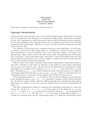
6. where
𝜋𝑛+1(𝑥) = (𝑥 − 𝑥0)(𝑥 − 𝑥1) ⋅ ⋅ ⋅ (𝑥 − 𝑥𝑛)
is a polynomial of degree 𝑛 + 1. Because 𝑥 is not one of the interpolation points, it follows that
𝜑(𝑡) has at least 𝑛 + 2 zeros: 𝑥, and the 𝑛 + 1 interpolation points 𝑥0, 𝑥1, . . . , 𝑥𝑛. Furthermore,
𝜋𝑛+1(𝑥) ∕= 0, so 𝜑(𝑡) is well-defined.
If 𝑓 is 𝑛+1 times continuously differentiable on an interval [𝑎, 𝑏] that contains the interpolation
points and 𝑥, then, by the Generalized Rolle’s Theorem, 𝜑(𝑛+1) must have at least one zero in [𝑎, 𝑏].
Therefore, at some point 𝜉(𝑥) in [𝑎, 𝑏], that depends on 𝑥, we have
0 = 𝜑(𝑛+1)
(𝜉(𝑥)) = 𝑓(𝑛+1)
(𝑡) −
𝑓(𝑥) − 𝑝𝑛(𝑥)
𝜋𝑛+1(𝑥)
(𝑛 + 1)!,
which yields the following result.
Theorem (Interpolation error) If 𝑓 is 𝑛 + 1 times continuously differentiable on [𝑎, 𝑏], and 𝑝𝑛(𝑥)
is the unique polynomial of degree 𝑛 that interpolates 𝑓(𝑥) at the 𝑛+1 distinct points 𝑥0, 𝑥1, . . . , 𝑥𝑛
in [𝑎, 𝑏], then for each 𝑥 ∈ [𝑎, 𝑏],
𝑓(𝑥) − 𝑝𝑛(𝑥) =
𝑛∏
𝑗=0
(𝑥 − 𝑥𝑗)
𝑓(𝑛+1)(𝜉(𝑥))
(𝑛 + 1)!
,
where 𝜉(𝑥) ∈ [𝑎, 𝑏].
It is interesting to note that the error closely resembles the Taylor remainder 𝑅𝑛(𝑥).
If the number of data points is large, then polynomial interpolation becomes problematic since
high-degree interpolation yields oscillatory polynomials, when the data may fit a smooth function.
Example Suppose that we wish to approximate the function 𝑓(𝑥) = 1/(1 + 𝑥2) on the interval
[−5, 5] with a tenth-degree interpolating polynomial that agrees with 𝑓(𝑥) at 11 equally-spaced
points 𝑥0, 𝑥1, . . . , 𝑥10 in [−5, 5], where 𝑥𝑗 = −5 + 𝑗, for 𝑗 = 0, 1, . . . , 10. Figure 1 shows that the
resulting polynomial is not a good approximation of 𝑓(𝑥) on this interval, even though it agrees
with 𝑓(𝑥) at the interpolation points. The following MATLAB session shows how the plot in the
figure can be created.
>> % create vector of 11 equally spaced points in [-5,5]
>> x=linspace(-5,5,11);
>> % compute corresponding y-values
>> y=1./(1+x.ˆ2);
>> % compute 10th-degree interpolating polynomial
>> p=polyfit(x,y,10);
>> % for plotting, create vector of 100 equally spaced points
>> xx=linspace(-5,5);
6

7. >> % compute corresponding y-values to plot function
>> yy=1./(1+xx.ˆ2);
>> % plot function
>> plot(xx,yy)
>> % tell MATLAB that next plot should be superimposed on
>> % current one
>> hold on
>> % plot polynomial, using polyval to compute values
>> % and a red dashed curve
>> plot(xx,polyval(p,xx),’r--’)
>> % indicate interpolation points on plot using circles
>> plot(x,y,’o’)
>> % label axes
>> xlabel(’x’)
>> ylabel(’y’)
>> % set caption
>> title(’Runge’’s example’)
In general, it is not wise to use a high-degree interpolating polynomial and equally-spaced interpo-
lation points to approximate a function on an interval [𝑎, 𝑏] unless this interval is sufficiently small.
The example shown in Figure 1 is a well-known example of the difficulty of high-degree polynomial
interpolation using equally-spaced points, and it is known as Runge’s example. □
Is it possible to choose the interpolation points so that the error is minimized? To answer this
question, we introduce the Chebyshev polynomials
𝑇𝑘(𝑥) = cos(𝑘 cos−1
(𝑥)),
which satisfy the three-term recurrence relation
𝑇𝑘+1(𝑥) = 2𝑥𝑇𝑘(𝑥) − 𝑇𝑘−1(𝑥), 𝑇0(𝑥) ≡ 1, 𝑇1(𝑥) ≡ 𝑥.
These polynomials have the property that ∣𝑇𝑘(𝑥)∣ ≤ 1 on the interval [−1, 1], while they grow
rapidly outside of this interval. Furthermore, the roots of these polynomials lie within the interval
[−1, 1]. Therefore, if the interpolation points 𝑥0, 𝑥1, . . . , 𝑥𝑛 are chosen to be the images of the roots
of the (𝑛 + 1)st-degree Chebyshev polynomial under a linear transformation that maps [−1, 1] to
[𝑎, 𝑏], then it follows that
𝑛∏
𝑗=0
(𝑥 − 𝑥𝑗) ≤
1
2𝑛
, 𝑥 ∈ [𝑎, 𝑏].
Therefore, the error in interpolating 𝑓(𝑥) by an 𝑛th-degree polynomial is determined entirely by
𝑓(𝑛+1).
7

8. Figure 1: The function 𝑓(𝑥) = 1/(1+𝑥2) (solid curve) cannot be interpolated accurately on [−5, 5]
using a tenth-degree polynomial (dashed curve) with equally-spaced interpolation points. This
example that illustrates the difficulty that one can generally expect with high-degree polynomial
interpolation with equally-spaced points is known as Runge’s example.
8