1. Chapter 3.4 Data Representation, Data Structures and Data Manipulation
3.4 (a) Numerical Representation
To turn a denary number into a binary number simply put the column headings, start
at the left hand side and follow the steps:
 If the column heading is less than the number, put a 1 in the column and then
subtract the column heading from the number. Then start again with the next
column on the right.
 If the column heading is greater than the number, put a 0 in the column and start
again with the next column on the right.
Note: You will be expected to be able to do this with numbers up to 255, because that
is the biggest number that can be stored in one byte of eight bits.
e.g. Change 117 (in denary) into a binary number.
Answer: Always use the column headings for a byte (8 bits)
128 64 32 16 8 4 2 1
Follow the algorithm.
128 is greater than 117 so put a 0 and repeat.
128 64 32 16 8 4 2 1
0
64 is less than 117 so put a 1.
128 64 32 16 8 4 2 1
0 1
Take 64 from 117 = 53, and repeat.
32 is less than 53, so put a 1.
128 64 32 16 8 4 2 1
0 1 1
Take 32 from 53 = 21, and repeat.
If you continue this the result (try it) is
128 64 32 16 8 4 2 1
0 1 1 1 0 1 0 1
So 117 (in denary) = 01110101 (in binary).
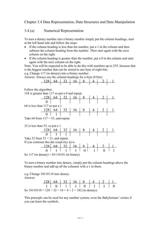
To turn a binary number into denary, simply put the column headings above the
binary number and add up all the columns with a 1 in them.
e.g. Change 10110110 into denary.
Answer:
128 64 32 16 8 4 2 1
1 0 1 1 0 1 1 0
So 10110110 = 128 + 32 + 16 + 4 + 2 = 182 (in denary).
This principle can be used for any number system, even the Babylonians’ sixties if
you can learn the symbols.
4.4 - 1

2. e.g. If we count in eights (called the OCTAL system) the column headings go up in
8’s.
512 64 8 1
So 117 (in denary) is 1 lot of 64, leaving another 53.
53 is 6 lots of 8 with 5 left over. Fitting this in the columns gives
512 64 8 1
0 1 6 5
So 117 in denary is 165 in octal.
Why bother with octal?
Octal and binary are related. If we take the three digits of the octal number 165 and
turn each one into binary using three bits each we get
1 = 001 6 = 110 5 = 101
Put them together and we get 001110101 which is the binary value of 117 which we
got earlier.
The value of this relationship is not important now, but it is the reason why octal is in
the syllabus.
Another system is called HEXADECIMAL (counting in 16’s). This sounds very
difficult, but it needn’t be, just use the same principles.
256 16 1
So 117 (in denary) is 7 lots of 16 (112) plus an extra 5. Fitting this in the columns
gives
256 16 1
0 7 5
Notice that 7 in binary is 0111 and that 5 is 0101, put them together and we get
01110101 which is the binary value of 117 again. So binary, octal and hexadecimal
are all related in some way.
There is a problem with counting in 16’s instead of the other systems. We need
symbols going further than 0 to 9 (only 10 symbols and we need 16!).
We could invent 6 more symbols but we would have to learn them, so we use 6 that
we already know, the letters A to F. In hexadecimal A stands for 10, B stands for 11
and so on to F stands for 15.
So a hexadecimal number BD stands for 11 lots of 16 and 13 units
= 176 + 13
= 189 ( in denary)
Note: B = 11, which in binary = 1011
D = 13, which in binary = 1101
Put them together to get 10111101 = the binary value of 189.
Binary Coded Decimal
Some numbers are not proper numbers because they don’t behave like numbers. A
barcode for chocolate looks like a number, and a barcode for sponge cake looks like a
number, but if the barcodes are added together the result is not the barcode for
chocolate cake. The arithmetic does not give a sensible answer. Values like this that
look like numbers but do not behave like them are often stored in binary coded
4.4 - 2

3. decimal (BCD). Each digit is simply changed into a four bit binary number which are
then placed after one another in order.
e.g. 398602 in BCD
Answer: 3 = 0011 9 = 1001
8 = 1000 6 = 0110
0 = 0000 2 = 0010
So 398602 = 001110011000011000000010 (in BCD)
Note: All the zeros are essential otherwise you can’t read it back.
3.4 (b) Negative Integers
Sign and Magnitude.
Use the first bit in the byte (the most significant bit (MSB)) to represent the sign (0
for + and 1 for -) instead of representing 128. This means that
+117 = 01110101 and -117 = 11110101
Notes: The range of numbers possible is now –127 to +127.
The byte does not represent just a number but also a sign, this makes arithmetic
difficult.
Two’s Complement
The MSB stays as a number, but is made negative. This means that the column
headings are
-128 64 32 16 8 4 2 1
+117 does not need to use the MSB, so it stays as 01110101.
-117 = -128 + 11
= -128 + (8 + 2 + 1) fitting this in the columns gives 10001011
Two’s complement seems to make everything more complicated for little reason at
the moment, but later it becomes essential for making the arithmetic easier.
3.4 (c) Binary Arithmetic
The syllabus requires the addition of two binary integers, and the ability to take one
away from another. The numbers and the answers will be limited to one byte.
Addition.
There are four simple rules 0+0=0
0+1=1
1+0=1
and the difficult one 1 + 1 = 0 (Carry 1)
e.g. Add together the binary equivalents of 91 and 18
Answer: 91 = 01011011
18 = 00010010 +
01101101 = 109
1 1
Subtraction.
This is where two’s complement is useful. To take one number away from another,
simply write the number to be subtracted as a two’s complement negative number and
then add them up.
e.g. Work out 91 – 18 using their binary equivalents.
Answer: 91 = 01011011
4.4 - 3

4. -18 as a two’s complement number is –128 + 110
= -128 +(+64 +32 +8 +4 +2)
= 11101110
Now add them 01011011
11101110 +
1 01001001
1 111111
But the answer can only be 8 bits, so cross out the 9th bit giving
01001001 = 64 + 8 + 1 = 73.
Notes: Lots of carrying here makes the sum more difficult, but the same rules are
used.
One rule is extended slightly because of the carries, 1+1+1 = 1 (carry 1)
Things can get harder but this is as far as the syllabus goes.
3.4 (d) Floating Point Representation
In the first part of this chapter we learned how to represent both positive and negative
integers in two's complement form. It is important that you understand this form of
representing integers before you learn how to represent fractional numbers.
In decimal notation the number 23.456 can be written as 0.23456 x 102. This means
that we need only store, in decimal notation, the numbers 0.23456 and 2. The number
0.23456 is called the mantissa and the number 2 is called the exponent. This is what
happens in binary.
For example, consider the binary number 10111. This could be represented by
0.10111 x 25 or 0.10111 x 2101. Here 0.10111 is the mantissa and 101 is the exponent.
Similarly, in decimal, 0.0000246 can be written 0.246 x 10-4. Now the mantissa is
0.246 and the exponent is –4.
Thus, in binary, 0.00010101 can be written as 0.10101 x 2-11 and 0.10101 is the
mantissa and –11 is the exponent.
It is now clear that we need to be able to store two numbers, the mantissa and the
exponent. This form of representation is called floating point form. Numbers that
involve a fractional part, like 2.46710 and 101.01012 are called real numbers.
3.4 (e) Normalising a Real Number
In the above examples, the point in the mantissa was always placed immediately
before the first non-zero digit. This is always done like this with positive numbers
because it allows us to use the maximum number of digits.
Suppose we use 8 bits to hold the mantissa and 8 bits to hold the exponent. The
binary number 10.11011 becomes 0.1011011 x 210 and can be held as
0 1 0 1 1 0 1 1 0 0 0 0 0 0 1 0
Mantissa Exponent
4.4 - 4

5. Notice that the first digit of the mantissa is zero and the second is one. The mantissa
is said to be normalised if the first two digits are different. Thus, for a positive
number, the first digit is always zero and the second is always one. The exponent is
always an integer and is held in two's complement form.
Now consider the binary number 0.00000101011 which is 0.101011 x 2-101. Thus the
mantissa is 0.101011 and the exponent is –101. Again, using 8 bits for the mantissa
and 8 bits for the exponent, we have
0 1 0 1 0 1 1 0 1 1 1 1 1 0 1 1
Mantissa Exponent
because the two's complement of –101, using 8 bits, is 11111011.
The reason for normalising the mantissa is in order to hold numbers to as high a
degree of accuracy as possible.
Care needs to be taken when normalising negative numbers. The easiest way to
normalise negative numbers is to first normalise the positive version of the number.
Consider the binary number –1011. The positive version is 1011 = 0.1011 x 2100 and
can be represented by
0 1 0 1 1 0 0 0 0 0 0 0 0 1 0 0
Mantissa Exponent
Now find the two's complement of the mantissa and the result is
1 0 1 0 1 0 0 0 0 0 0 0 0 1 0 0
Mantissa Exponent
Notice that the first two digits are different.
As another example, change the decimal fraction –11/32 into a normalised floating
point binary number.
11/32 = 1/4 + 1/16 + 1/32 = 0.01 + 0.0001 + 0.00001 = 0.01011
= 0.1011 x 2-1
Therefore –11/32 = -0.1011 x 2-1
Using two's complement –0.1011 is 1.0100 and –1 is 11111111
and we have
4.4 - 5

6. 1 0 1 0 0 0 0 0 1 1 1 1 1 1 1 1
Mantissa Exponent
The fact that the first two digits are always different can be used to check for invalid
answers when doing calculations.
3.4 (f) Accuracy and Range
The smallest positive mantissa is 0.1000000 and the smallest exponent is 10000000.
This represents
0.1000000 x 210000000 = 0.1000000 x 2-128
which is very close to zero; in fact it is 2-129.
The largest negative number (i.e. the negative number closest to zero) is
1.0111111 x 210000000 = -0.1000001 x 2-128
Note that we cannot use 1.1111111 for the mantissa because it is not normalised. The
first two digits must be different.
The smallest negative number (i.e. the negative number furthest from zero) is
1.0000000 x 201111111 = -1.0000000 x 2127 = -2127.
NOTE: reducing the size of the mantissa reduces the accuracy, but we have a much
greater range of values as the exponent can now take larger values.
3.4 (g) Static and Dynamic Data Structures
Static data structures are those structures that do not change in size while the program
is running. A typical static data structure is an array because once you declare its size,
it cannot be changed. (In fact, there are some languages that do allow the size of
arrays to be changed in which case they become dynamic data structures.)
Dynamic data structures can increase and decrease in size while a program is running.
A typical example is a linked list.
The following table gives advantages and disadvantages of the two types of data
structure.
4.4 - 6

7. Advantages Disadvantages
Static structures Compiler can allocate Programmer has to
space during compilation. estimate the maximum
amount of space that is
Easy to program. going to be needed.
Easy to check for Can waste a lot of space.
overflow.
An array allows random
access.
Dynamic structures Only uses the space Difficult to program.
needed at any time.
Can be slow to implement
Makes efficient use of searches.
memory.
A linked list only allows
Storage no longer required serial access.
can be returned to the
system for other uses.
3.4 (h) Algorithms
Linked Lists - Insertion
The algorithm must check for an empty free list as there is then no way of adding new
data. It must also check to see if the new data is to be inserted at the front of the list.
If neither of these are needed, the algorithm must search the list to find the position
for the new data. The algorithm is given below.
1. Check that the free list is not empty.
2. If it is empty report an error and stop.
3. Set NEW to equal FREE.
4. Remove the node from the stack by setting FREE to pointer in cell pointed to
by FREE.
5. Copy data into cell pointed to by NEW.
6. Check for an empty list by seeing if HEAD is NULL
7. If HEAD is NULL then
a. Pointer in cell pointed to by NEW is set to NULL
b. Set HEAD to NEW and stop.
8. If data is less than data in first cell THEN
a. Set pointer in cell pointed to by NEW to HEAD.
b. Set HEAD to NEW and stop
9. Search list sequentially until the cell found is the one immediately before the
new cell that is to be inserted. Call this cell PREVIOUS.
10. Copy the pointer in PREVIOUS into TEMP.
11. Make the pointer in PREVIOUS equal to NEW
12. Make the pointer in the cell pointed to by NEW equal to TEMP and stop.
4.4 - 7

8. Linked Lists - Deletion
In this case, the algorithm must make sure that there is something in the list to delete.
1. Check that the list is not empty.
2. If the list is empty report an error and stop.
3. Search list to find the cell immediately before the cell to be deleted and call it
PREVIOUS.
4. If the cell is not in the list, report an error and stop.
5. Set TEMP to pointer in PREVIOUS.
6. Set pointer in PREVIOUS equal to pointer in cell to be deleted.
7. Set pointer in cell to be deleted equal to FREE.
8. Set FREE equal to TEMP and stop.
Linked Lists - Amendment
Amendments can be done by searching the list to find the cell to be amended.
The algorithm is
1. Check that the list is not empty.
2. If the list is empty report an error and stop.
3. Search the list to find the cell to be amended.
4. Amend the data but do not change the key.
5. Stop.
Linked Lists - Searching
Assuming that the data in a linked list is in ascending order of some key value, the
following algorithm explains how to find where to insert a cell containing new data
and keep the list in ascending order. It assumes that the list is not empty and the data
is not to be inserted at the head of the list.
Set POINTER equal to HEAD
REPEAT
Set NEXT equal to pointer in cell pointed to by POINTER
If new data is less than data in cell pointed to by POINTER then set POINTER equal
to NEXT
UNTIL
Note: A number of methods have been shown here to describe algorithms associated
with linked lists. Any method is acceptable provided it explains the method. An
algorithm does not have to be in pseudo code, indeed, the sensible way of explaining
these types of algorithm is often by diagram.
4.4 - 8

9. Stacks – Insertion
The algorithm for insertion is
1. Check to see if stack is full.
2. If the stack is full report an error and stop.
3. Increment the stack pointer.
4. Insert new data item into cell pointed to by the stack pointer and stop.
Stacks – Deletion
When an item is deleted from a stack, the item's value is copied and the stack pointer
is moved down one cell. The data itself is not deleted. This time, we must check that
the stack is not empty before trying to delete an item.
The algorithm for deletion is
1. Check to see if the stack is empty.
2. If the stack is empty report an error and stop.
3. Copy data item in cell pointed to by the stack pointer.
4. Decrement the stack pointer and stop.
These are the only two operations you can perform on a stack.
Queues - Insertion
The algorithm for insertion is
1. Check to see if queue is full.
2. If the queue is full report an error and stop.
3. Insert new data item into cell pointed to by the head pointer.
4. Increment the head pointer and stop.
Queues - Deletion
Before trying to delete an item, we must check to see that the queue is not empty.
Using the representation above, this will occur when the head and tail pointers point
to the same cell.
The algorithm for deletion is
1. Check to see if the queue is empty.
2. If the queue is empty report error and stop.
3. Copy data item in cell pointed to by the tail pointer.
4. Increment tail pointer and stop.
4.4 - 9

10. These are the only two operations that can be performed on a queue.
3.4 (i) Algorithms for Trees
Trees - Insertion
To add a new value, we look at each node starting at the root. If the new value is less
than the value at the node move left, otherwise move right. Repeat this for each node
arrived at until there is no node. Insert a new node at this point and enter the data.
Now let's try putting "Jack Spratt could eat no fat" into a tree. Jack must be the root
of the tree. Spratt comes after Jack so go right and enter Spratt. could comes before
Jack, so go left and enter could. eat is before Jack so go left, it's after could so go
right. This is continued to produce the tree in Fig. 3.4.i.1.
Jack
could Spratt
eat no
fat
Fig. 3.4.i.1
The algorithm for this is
1. If tree is empty enter data item at root and stop.
2. Current node = root.
3. Repeat steps 4 and 5 until current node is null.
4. If new data item is less than value at current node go left else go right.
5. Current node = node reached (null if no node).
6. Create new node and enter data.
4.4 - 10

11. Using this algorithm and adding the word and we follow these steps.
1. The tree is not empty so go to the next step.
2. Current node contains Jack.
3. Node is not null.
4. and is less than Jack so go left.
5. Current node contains could.
3. Node is not null.
4. and is less than could so go left.
5. Current node is null.
3. Current node is null so exit loop.
6. Create new node and insert and and stop.
We now have the tree shown in Fig. 3.4.i.2.
Jack
could Spratt
and eat no
fat
Fig. 3.4.i.2
If the values are read from the left to the right, using the algorithm
Follow left subtree
Read node
Follow right subtree
Return
The values can be read in order. There are many different ways of reading the values
from a tree, but the simplest is the one illustrated by the dashed line in the diagram
above. It is also the only way that you will be asked to read a tree in an examination.
The diagram with the dashed line would be read as
Could, Eat, Fat, Jack, No, Spratt
Note that the words are now in alphabetic order.
4.4 - 11

12. 3.4 (j) Searching Methods
Serial Search
Let the data consist of n values held in an array called DataArray which has subscripts
numbered from 1 upwards. Let X be the value we are trying to find. We must check
that the array is not empty before starting the search.
The algorithm to find the position of X is
1. If n < 1 then report error, array is empty.
2. For i = 1 to n do
a. If DataArray[i] = X then return i and stop.
3. Report error, X is not in the array and stop.
Note that the for loop only acts on the indented line. If there is more than one
operation to perform inside a loop, make sure that all the lines are indented.
Binary Search
Assume that the data is held in an array as described above but that the data is in
ascending order in the array. We must split the lists in two. If there is an even
number of values, dividing by two will give a whole number and this will tell us
where to split the list. However, if the list consists of an odd number of values we
will need to find the integer part of it, as an array subscript must be an integer.
We must also make sure that, when we split a list in two, we use the correct one for
the next search. Suppose we have a list of eight values. Splitting this gives a list of
the four values in cells 1 to 4 and four values in cells 5 to 8. When we started we
needed to consider the list in cells 1 to 8. That is the first cell was 1 and the last cell
was 8. Now, if we move into the first list (cells 1 to 4), the first cell stays at 1 but the
last cell becomes 4. Similarly, if we use the second list (cells 5 to 8), the first cell
becomes 5 and the last is still 8. This means that if we use the first list, the first cell in
the new list is unchanged but the last is changed. However, if we use the second list,
the first cell is changed but the last is not changed. This gives us the clue of how to
do the sort.
3.4 (k) Sorting and Merging
Sorting is placing values in an order such as numeric order or alphabetic order. The
order may be ascending or descending. For example the values
3 5 6 8 12 16 25
are in ascending numeric order and
Will Rose Mattu Juni Hazel Dopu Anne
are in descending alphabetic order.
4.4 - 12

13. Merging is taking two lists which have been sorted into the same order and putting
them together to form a single sorted list. For example, if the lists are
Bharri Emi Kris Mattu Parrash Roger Will
and
Annis Chu Liz Medis Ste
when merged they become
Annis Bharri Chu Emi Kris Liz Mattu Medis Parrash Roger Ste Will
There are many methods that can be used to sort lists. You only need to understand
two of them. These are the insertion sort and the merge sort. This Section describes
the two sorts and a merge in general terms; the next Section gives the algorithms.
Insertion Sort
In this method we compare each number in turn with the numbers before it in the list.
We then insert the number into its correct position.
Consider the list
20 47 12 53 32 84 85 96 45 18
We start with the second number, 47, and compare it with the numbers preceding it.
There is only one and it is less than 47, so no change in the order is made. We now
compare the third number, 12, with its predecessors. 12 is less than 20 so 12 is
inserted before 20 in the list to give the list
12 20 47 53 32 84 85 96 45 18
This is continued until the last number is inserted in its correct position. In Fig.
3.4.k.1 the blue numbers are the ones before the one we are trying to insert in the
correct position. The red number is the one we are trying to insert.
20 47 12 53 32 84 85 96 45 18 Original list, start with second
number.
20 47 12 53 32 84 85 96 45 18 No change needed.
53 32 84 85 96 45 18 Now compare 12 with its
predecessors.
12 20 47 53 32 84 85 96 45 18 Insert 12 before 20.
12 20 47 53 32 84 85 96 45 18 Move to next value.
12 20 47 53 32 84 85 96 45 18 53 is in the correct place.
12 20 47 53 32 84 85 96 45 18 Move to the next value.
12 20 32 47 53 84 85 96 45 18 Insert it between 20 and 47
12 20 32 47 53 84 85 96 45 18 Move to the next value.
4.4 - 13

14. 12 20 32 47 53 84 85 96 45 18 84 is in the correct place.
12 20 32 47 53 84 85 96 45 18 Move to the next value.
12 20 32 47 53 84 85 96 45 18 85 is in the correct place.
12 20 32 47 53 84 85 96 45 18 Move to the next value.
12 20 32 47 53 84 85 96 45 18 96 is in the correct place.
12 20 32 47 53 84 85 96 45 18 Move to the next value.
12 20 32 45 47 53 84 85 96 18 Insert 45 between 32 and 47.
12 20 32 45 47 53 84 85 96 18 Move to the next value.
12 18 20 32 45 47 53 84 85 96 Insert 18 between 12 and 20.
Fig. 3.4.k.1
Merging
Consider the two sorted lists
2 4 7 10 15 and 3 5 12 14 18 26
In order to merge these two lists, we first compare the first values in each list, that is 2
and 3. 2 is less than 3 so we put it in the new list.
New = 2
Since 2 came from the first list we now use the next value in the first list and compare
it with the number from the second list (as we have not yet used it). 3 is less than 4 so
3 is placed in the new list.
New = 2 3
As 3 came from the second list we use the next number in the second list and compare
it with 4. This is continued until one of the lists is exhausted. We then copy the rest
of the other list into the new list. The full merge is shown in Fig. 3.4.k.2.
First List Second List New List
2 4 7 10 15 3 5 12 14 18 26 2
2 4 7 10 15 3 5 12 14 18 26 2 3
2 4 7 10 15 3 5 12 14 18 26 2 3 4
2 4 7 10 15 3 5 12 14 18 26 2 3 4 5
2 4 7 10 15 3 5 12 14 18 26 2 3 4 5 7
2 4 7 10 15 3 5 12 14 18 26 2 3 4 5 7 10
2 4 7 10 15 3 5 12 14 18 26 2 3 4 5 7 10 12
2 4 7 10 15 3 5 12 14 18 26 2 3 4 5 7 10 12 14
2 4 7 10 15 3 5 12 14 18 26 2 3 4 5 7 10 12 14 15
2 4 7 10 15 3 5 12 14 18 26 2 3 4 5 7 10 12 14 15 18
2 4 7 10 15 3 5 12 14 18 26 2 3 4 5 7 10 12 14 15 18 26
Fig. 3.4.k.2
4.4 - 14

15. 4.4 - 15