Data Presenetation
•Download as PPTX, PDF•
0 likes•278 views

In this lesson we enrich what the students have already learned from Grade 1 to 10 about presenting data. Additional concepts could help the students to appropriately describe further the data set.

Recommended
More Related Content
What's hot
What's hot (20)
Similar to Data Presenetation
Similar to Data Presenetation (20)
More from Samuel John Parreño
Recently uploaded
Recently uploaded (20)
Data Presenetation
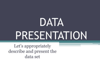
- 1. DATA PRESENTATION Let’s appropriately describe and present the data set
- 2. Learning Outcomes At the end of the lesson, the learner is able to identify and use the appropriate method of presenting information from a data set effectively.
- 3. Textual or Narrative, Tabular and Graphical Method of Presentation
- 4. TEXTUAL/PARAGRAPH/NARRATIVE FORM • One describes the data by enumerating some of the highlights of the data set like giving the highest, lowest or the average values. • In case there are only few observations, say less than ten observations, the values could be enumerated if there is a need to do so.
- 5. Example The country’s poverty incidence among families as reported by the Philippine Statistics Authority (PSA), the agency mandated to release official poverty statistics, decreases from 21% in 2006 down to 19.7% in 2012. For 2012, the regional estimates released by PSA indicate that the Autonomous Region of Muslim Mindanao (ARMM) is the poorest region with poverty incidence among families estimated at 48.7%. The region with the smallest estimated poverty incidence among families at 2.6% is the National Capital Region (NCR)
- 6. TABULAR • applicable for large data sets. • Trends could easily be seen in this kind of presentation. • However, there is a loss of information when using such kind of presentation. • The frequency distribution table is the usual tabular form of presenting the distribution of the data.
- 7. COMMON PARTS OF STATISTICAL TABLE a. Table title includes the number and a short description of what is found inside the table. b. Column header provides the label of what is being presented in a column. c. Row header provides the label of what is being presented in a row. d. Body are the information in the cell intersecting the row and the column.
- 8. •a table should have at least three rows and/or three columns. •too many information to convey in a table is also not advisable. •Tables are usually used in written technical reports and in oral presentation.
- 10. GRAPHICAL PRESENTATION • a visual presentation of the data. • commonly used in oral presentation. • There are several forms of graphs to use like the pie chart, pictograph, bar graph, line graph, histogram and box-plot. Which form to use depends on what information is to be relayed. For example, trends across time are easily seen using a line graph. • However, values of variables in nominal or ordinal levels of measurement should not be presented using line graph. Rather a bar graph is more appropriate to use.
- 17. The FDT • An FDT is a presentation containing non-overlapping categories or classes of a variable and the frequencies or counts of the observations falling into the categories or classes. There are two types of FDT according to the type of data being organized: a qualitative FDT or a quantitative FDT.
- 18. Two Types of FDT according to the type of data being organized: 1. Qualitative FDT • the non-overlapping categories of the variable are identified, and frequencies, as well as the percentages of observations falling into the categories, are computed. 2. Quantitative FDT • two types: ungrouped and grouped FDT.
- 19. Qualitative Data FDT (example)
- 20. Qualitative Data Bar graph (example)
- 21. Two Types of Quantitative FDT 1. Ungrouped FDT • is constructed when there are only a few observations or if the data set contains only few possible values. 2. Grouped FDT • is constructed when there is a large number of observations and when the data set involves many possible values. The distinct values are grouped into class intervals.
- 22. Example 55 70 57 73 55 59 64 72 60 48 58 54 69 51 63 78 75 64 65 57 71 78 76 62 49 66 62 76 61 63 63 76 52 76 71 61 53 56 67 71
- 23. Steps in the construction of a grouped FDT 1. Identify the largest data value or the maximum (MAX) and smallest data value or the minimum (MIN) from the data set and compute the range, R. The range is the difference between the largest and smallest value, i.e. R = MAX – MIN. 2. Determine the number of classes, k using 𝑘 = 𝑁, where N is the total number of observations in the data set. Round-off k to the nearest whole number. It should be noted that the computed k might not be equal to the actual number of classes constructed in an FDT.
- 24. 3. Calculate the class size, c, using c = R/k. Round off c to the nearest value with precision the same as that with the raw data. 4. Construct the classes or the class intervals. A class interval is defined by a lower limit (LL) and an upper limit (UL). The LL of the lowest class is usually the MIN of the data set. The LL’s of the succeeding classes are then obtained by adding c to the LL of the preceding classes. The UL of the lowest class is obtained by subtracting one unit of measure 1 10 𝑥 , where x is the maximum number of decimal places observed from the raw data) from the LL of the next class. The UL’s of the succeeding classes are then obtained by adding c to the UL of the preceding classes. The lowest class should contain the MIN, while the highest class should contain the MAX.
- 25. 5. Tally the data into the classes constructed in Step 4 to obtain the frequency of each class. Each observation must fall in one and only one class. 6. Add (if needed) the following distributional characteristics: a. True Class Boundaries (TCB). The TCBs reflect the continuous property of a continuous data. It is defined by a lower TCB (LTCB) and an upper TCB (UTCB). These are obtained by taking the midpoints of the gaps between classes or by using the following formulas: LTCB = LL – 0.5(one unit of measure) and UTCB = UL + 0.5(one unit of measure)
- 26. b. Class Mark (CM). The CM is the midpoint of a class and is obtained by taking the average of the lower and upper TCB’s, i.e. CM = (LTCB + UTCB)/2. c. Relative Frequency (RF). The RF refers to the frequency of the class as a fraction of the total frequency, i.e. RF = frequency/N. RF can be computed for both qualitative and quantitative data. RF can also be expressed in percent. d. Cumulative Frequency (CF). The CF refers to the total number of observations greater than or equal to the LL of the class (>CF) or the total number of observations less than or equal to the UL of the class (<CF)
- 27. e. Relative Cumulative Frequency (RCF). RCF refers to the fraction of the total number of observations greater than or equal to the LL of the class (>RCF) or the fraction of the total number of observations less than or equal to the UL of the class (<RCF). Both the <RCF and >RCF can also be expressed in percent.
- 29. The histogram is a graphical presentation of the frequency distribution table in the form of a vertical bar graph. There are several forms of the histogram and the most common form has the frequency on its vertical axis while the true class boundaries in the horizontal axis. As an example, the FDT and its corresponding histogram of the 2012 estimated poverty incidences of 144 municipalities and cities of Region VIII are shown
- 31. Key Points • Three methods of data presentation: textual, tabular and graphical • Two or all the methods could be combined to fully describe the data at hand. • Distribution of data is presented using frequency distribution table and histogram.