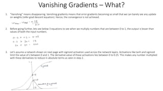
1.
Vanishing Gradients – What?
1. “Vanishing” means disappearing. Vanishing gradients means that error gradients becoming so small that we can barely see any update
on weights (refer grad descent equation). Hence, the convergence is not achieved.
2. Before going further, lets see below 3 equations to see when we multiply numbers that are between 0 to 1, the output is lesser than
values of both the input numbers.
3. Let’s assume a network shown on next page with sigmoid activation used across the network layers. Activations like tanh and sigmoid
limit the value of z between 0 and 1. The derivative value of these activations lies between 0 to 0.25. This makes any number multiplied
with these derivatives to reduce in absolute terms as seen in step 2.

2.
Vanishing Gradients

3.
Vanishing Gradients – How to Avoid?
1. Reason  Let’s see the equation for gradient of error w.r.t w17 and gradient of error w.r.t w23. The number of items required to be
multiplied to calculate gradient of error w.r.t w17 (a weight in initial layer) is way more than number of items required to be multiplied to
calculate gradient of error w.r.t w23 (a weight in later layers). Now, the terms in these gradients that do partial derivative of activation will
be valued between 0 to 0.25 (refer point 3). Since number of terms less than 1 is more for error gradients in initial layers, hence,
vanishing gradient effect is seen more prominently in the initial layers of network. The number of terms required to compute gradient
w.r.t w1, w2 etc. will be quite high.
Resolution  The way to avoid the chances of a vanishing gradient problem is to use activations whose derivative is not limited to values less
than 1. We can use Relu activation. Relu’s derivative for positive values is 1. The issue with Relu is it’s derivative for negative values is 0 which
makes contribution of some nodes 0. This can be managed by using Leaky Relu instead.

4.
Vanishing Gradients – How to Avoid?

5.
Vanishing Gradients – How to Avoid?
2. Reason  The first problem that we discussed was the usage of activations whose derivatives are low. The second problem deals with
low value of initialized weights. We can understand this from simple example as shown in network on previous page. The equations for
error grad w.r.t w1 includes value of w5 as well. Hence, if value of w5 is initialized very low, it will also plays a role in making the gradient
w.r.t w1 smaller i.e vanishing gradient.
We can also say Vanishing gradient problems will be more prominent in deep networks. This is because the number of multiplicative terms to
compute the gradient of initial layers in a deep network is very high.
Resolution  As we can see from below equations, the derivative of activation function along with weights play a role in causing vanishing
gradients because both are there in equation for computation of error gradient. We need to initialize the weights properly to avoid vanishing
gradient problem. We will discuss about it further in weight initialization strategy section.

6.
Exploding Gradients – What?
1. “Exploding” means increasing to a large extent. Exploding gradients means that error gradients becoming so big that the update on
weights is too high in every iteration. This causes the weights to swindle a lot and causes error to keep missing the global minima. Hence,
the convergence becomes tough to be achieved.
2. Exploding gradients are caused due to usage of bigger weights used in the network.
3. Probable resolutions
1. Keep low learning rate to accommodate for higher weights
2. Gradient clipping
3. Gradient scaling
4. Gradient scaling
1. For every batch, get all the gradient vectors for all samples.
2. Find L2 norm of the concatenated error gradient vector.
1. If L2 norm > 1 (1 is used as an example here)
2. Scale/normalize the gradient terms such that L2 norm becomes 1
3. Code example  opt = SGD(lr=0.01, momentum=0.9, clipnorm=1.0)
5. Gradient clipping
1. For every sample in a batch, if the gradient value w.r.t any weight is outside a range (let’s say -0.5 <= gradient_value <= 0.5), we clip
the gradient value to the border values. If gradient value is 0.6, we clip it to make it 0.5.
2. Code example  opt = SGD(lr=0.01, momentum=0.9, clipvalue=0.5)
6. Generic practice is to use same values of clipping / scaling throughout the network.