2. 10
basin and 44–244 mm for the Kompienga dam
basin. Moon et al. 2004 applied a modified WTF
and statistical analysis of groundwater hydrographs
to estimate groundwater recharge for a river basin
of South Korea. The average recharge ratios of the
monitoring stations, grouped according to their
groundwater hydrographs, varied from 4.07 to
15.29%. Rasoulzadeh & Moosavi 2008 by using an
inverse approach and considering the WTF model
as a forward model estimated the groundwater
recharge and WTF parameters for the vicinity of
Tashk Lake (called Tavabe-e-Arsanjan) in Iran,
Fars province. Ganji khorramdel et al. 2008 used
Double Water Table Fluctuation to optimize an
observation well network in order to estimate the
groundwater budget of Astane-Koochesfahan
aquifer in Iran, Gilan Province. The results showed
that such an optimized network provides far fewer
measurement points, i.e. 33 wells, without consid-
erably changing the conclusions regarding ground-
water budget.
In this research the Hydrological Budget method
(HB) was applied by Geographical Information
System (GIS) technique to estimate annual aver-
age groundwater recharge of the whole study area
(Neishaboor Plain). The monthly groundwater
recharge for each Thiessen polygon was estimated
using Distributed Hydrological Budget (DHB).
Moreover the WTF method and an inverse mod-
eling approach was implemented to determine
how much of precipitation and irrigation return
flow contribute to natural groundwater recharge in
monthly scale.
2 MATERIALS AND METHODS
2.1 Description of the study area
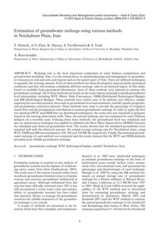
The Neishaboor plain is located between 35°40′ N
to 36°39′ N latitude and 58°17′ E to 59°30′ E longi-
tude with semi-arid to arid climate, in the northeast
of Iran as shown in Figure 1. The total geographi-
cal area is 7,350 km2
, consisting of 3,160 km2
mountainous terrain and about 4,190 km2
of plain.
The maximum elevation is located in the Binalood
Mountains (3,300 m above sea level), and the mini-
mum elevation is at the outlet of the plain (Hosein
Abad Jangal) at 1,050 m above mean sea level.
The average annual precipitation is 234 mm, but
this varies considerably from one year to another.
The mean annual temperatures at the Bar-Aria
station (in the mountainous area) and Moham-
mad Abad-Fedisheh station (in the plain area) are
13 and 13.8°C, respectively. The annual potential
evapotranspiration is about 2,335 mm (Velayati
and Tavassloi 1991). According to official reports,
about 93.5% of the withdrawals in the Neishaboor
Figure 1. Location of study area in Iran, Khorasan-
Razavi province.
watershed are consumed by agriculture, mostly in
irrigation.
Moreover, the share of surface-water resources
in total consumption is about 4.2%. It means
that groundwater is a primary source of water
for different purposes and surface water plays a
minor role in providing water supply services in
the Neishaboor watershed. Therefore, crop eva-
potranspiration (ETc)—evapotranspiration from
disease-free, well fertilized crops, grown in large
fields, under optimum soil water conditions, and
achieving full reduction under the given climatic
conditions—is responsible for about 90% of water-
resources consumption (Hoseini et al. 2005).
2.2 Theory of Hydrological Budget (HB) method
The hydrologic budget for a geographic basin can
be written as:
(W|Qin)(ETROIPQbfQout) Qw = ΔS (1)
where W is the applied water on the ground sur-
face; Qin and Qout are subsurface water fluxes into
and out of a geographic basin along a boundary;
ET represents evapotranspiration losses in surface
and subsurface waters, including the unsaturated
and saturated zones; RO is surface water runoff;
IP is intercepted precipitation by vegetation; Qbf
is groundwater discharge to streams (baseflow);
3. 11
Qw is groundwater withdrawal through pumping
wells; and ΔS is the change in saturated ground-
water storage. The units for all components in the
hydrologic budget equation are in volume per time
period.
As groundwater recharge includes any percolated
water that reaches the saturated portion of the water
table aquifer per time period, and can be written as:
Rt = W − (ET + RO + IP + Qbf + Qin − Qout) (2)
where Rt is groundwater recharge.
Assuming water table aquifer conditions, the
change in groundwater storage per time period can
be written (Bredehoeft et al. 1982) as:
ΔS − ΔH × Agb × Sy (3)
where ΔH is the average change of the measured
groundwater levels per time period; Agb is the area
of the geographic basin; and Sy is the average spe-
cific yield of the water table aquifer.
Substituting Equations 2 and 3 into Equation 1
and simplifying results in:
Rt = Qw + (ΔH × Agb × Sy) (4)
If the geographic basin area is divided into a grid,
then the groundwater recharge per time period, Rt,
equals the summation of groundwater recharge of
the grid, and can be presented as:
RtRR i
n
i
n
( )h a Sih i yS i×hihh∑ ∑r Qirri
n
QQ=rirr=1 1i=i∑Qirr QQi wQ (5)
where ri, Δhi, ai, n and Syi represent the associated
quantity for each grid cell and n is the number of
grid cells. The effect of groundwater withdrawal is
assumed to be equally distributed on the grid. Any
time period may be used, but for semi-arid regions
where groundwater levels are very deep, it is best
to assume a longer time period (for example 1 year
time period) because of the lag time necessary for
groundwater recharge to reach the saturated water
table system (Manghi et al. 2009).
2.3 Theory of Distributed Hydrological Budget
(DHB) method
The groundwater recharge can be estimated by clas-
sifying the study area into Thiessen polygons based
upon observation wells and writing the water budget
equation (Eq. 1) for each Thiessen polygon. The
groundwater recharge for each Thiessen polygon in
monthly scale is estimated from the Equation 6, i.e.,
Rt = Qw + (ΔH × Agh × Sy) − (Qin − Qout) − ET − Qbf
(6)
Since the groundwater depth in the study area is
more than 5 meters and there is no river to drain
the groundwater, the terms ET and Qbf were negli-
gible in the study area.
2.4 Theory of Water Table Fluctuation (WTF)
method
The water table fluctuation method by analyzing
water level fluctuations provides an estimate of
groundwater recharge. For applying this method
only groundwater level and specific yield data are
needed. The WTF method is based on the premise
that rises in groundwater levels in unconfined aqui-
fers are due to recharge water arriving at the water
table. Recharge is calculated as (Healy & Cook
2002):
R = Sydh/dt = SyΔh/Δt (7)
Where R is recharge; Sy is specific yield; h is water-
table height, and t is time.
To derive Equation 7 one needs to assume that
water arriving at the water table goes immediately
into storage and that all other components of
Equation 1 are zero during the period of recharge.
A time lag occurs between the arrival of water dur-
ing a recharge event and the redistribution of that
water to the other components of Equation 1. If
the method is applied during that time lag, all of
the water going into recharge can be accounted for.
This assumption is most valid over short periods
of time, and it is this time frame for which applica-
tion of the method is most appropriate (Healy &
Cook 2002; Scanlon et al. 2002).
2.4.1 Inverse modeling approach
The Equation 7 could be rewritten as below:
dh/dt = R/Sy (8)
The above equation considers the groundwater
recharge as a whole. Recharge might be resulted
from precipitation (P), irrigation return flow
(QIrrigation) and net subsurface water flux (QInOut) into
the aquifer or Thiessen polygon. The Equation 8 is
rearranged as the following equation by consider-
ing these parameters within it:
dh
dt
irrigation pumpage InOut
= + − +
pumpageβ λPβ
S
Qiλλ
S
Qp
S
QI
Sy yS S y yS S
(9)
where λ = percentage of irrigation return flow
which contributes to recharge; β = percentage of
precipitation which contributes to recharge; and
4. 12
QPumpage = groundwater withdrawal through pump-
ing wells (Rasoulzadeh & Moosavi 2008).
InversemodelingapproachconsidersWTFmodel
as forward model and fits Equation 9 on observed
data, then unknown parameters of WTF model
are estimated with the help of one of optimization
procedure in order to minimize objective function
(difference between observed and simulated water
level fluctuations with WTF model) (Eq. 10).
RMSE
x x f x x x
n
n nx
=
−∑ ( (F , , )xn ,x ))1 2x,x x, 2
… ff, )xn xx xx,
(10)
where F = observed values; f = simulated values;
and n = the number of observed values.
The optimization procedure was used with the
help of Spss 18.0 to minimize Root Mean Square
Error (RMSE) and to get the best fit between the
two curves. Spss uses Levenberg–Marquardt and
Sequential Quadratic Programming to minimize
objective function.
2.5 Conceptual model of study area
To build conceptual model and preparing required
data, at first point shape file of Observation Wells
(OWs) added to ARCMAP (ARCGIS products)
and Thiessen polygon were made based on them.
Figure 2 illustrates the conceptual model of study
area and Thiessen polygons.
Following the construction of Thiessen poly-
gons based on observation wells, the monthly
records of groundwater levels at each polygon were
arranged at 35 Excel spreadsheets for the period
from October 2000 to September 2010. Then,
monthly records of rainfall, net subsurface water
flux and Abstraction Wells (AWs) data were listed
against the corresponding groundwater level data
for each sub-zone, and plotted against time.
Monthly net subsurface water fluxes were esti-
mated using Darcy Flow function of ARCGIS.
Monthly groundwater level, monthly saturation
thickness (i.e., subtraction of bed rock and ground-
water level rasters), the porosity and transmissiv-
ity rasters are required for calculating groundwater
flow across grid cells using the Darcy Flow function.
These rasters were produced with Topo to Raster
embedded in ARCGIS 9.3 3D Analyst function by
pixcel size of 1000 by 1000 m. Monthly Darcy Flow
outputs were summed for each sub-zone.
Since, the Darcy Flow function could not cal-
culate the in/outflow for the boundary cells, the
monthly lateral groundwater inflow and outflows
were calculated by using Equation 11 as (Fig. 3):
Q j
T T
h h
x
yxQQ
i j i j
i jTT i jTT
i jhh i jhh
( ,i ) *
( )Ti jTT ( )Ti jTTj i)j ( i
j i
j i
j, )1
2
1
2
Δ
Δyy
(11)
where Qx = lateral groundwater inflow or out-
flow; T = transmissivity; h = groundwater level;
i and j = represents each cell position at x and y
directions, respectively; Δx = distance between two
adjacent cell; and Δy = width of each cell. These
lateral inflow or outflows were summed up by the
net subsurface water fluxes which estimated for the
boundary polygons.
For spatial distribution of rainfall in the study
area the Inverse Distance Weighting method (IDW)
was applied, then the monthly records of rainfall
at each polygon were averaged to be used with
DHB and WTF models. Groundwater withdrawals
through pumping wells are used for irrigation pur-
poses. So the monthly records of abstraction wells
were summed for each polygon.
3 RESULTS AND DISCUSSION
For calculating groundwater recharge using the
HB method (Eq. 5), the rasters of groundwater
level of October and September of each year wasFigure 2. Conceptual model of the study area.
Figure3. Thispictureillustratesthathowthelateralground-
water inflow or outflow were calculated in boundaries.
5. 13
subtracted to calculate Δhi in each pixel (grid cell).
The raster of specific yield was also used to com-
pute the change in saturated groundwater storage.
Then annual average groundwater recharge rate
based on Equation (5) for Neishaboor Plain was
estimated from 2000 to 2010 (Table 1).
The average contribution of groundwater
recharge for a ten-year period was about 61% of the
totalgroundwaterwithdrawal(Table1).Theaverage
groundwater extraction from the Neishaboor Plain
from 2000 to 2010 was 649 MCM. Therefore,
39% of exploitation was supplied from saturated
groundwater storage and 61% was the result of
groundwater recharge including net groundwater
inflow, infiltration and irrigation return flow. If we
subtract the net groundwater inflow (which equals
41 MCM based on Table 4) from annual average
Table 1. Estimated groundwater recharge (MCM) for
Neishaboor Plain form 2000/2001 to 2009/2010.
Time
period (Year)
Qw
(MCM)
ΔS
(MCM)
Rt
(MCM)
Rt
(%)
2000–2001 690 −379 311 45
2001–2002 679 −308 371 55
2002–2003 671 −204 467 70
2003–2004 663 −274 390 59
2004–2005 654 −227 427 65
2005–2006 643 −251 392 61
2006–2007 633 −216 417 66
2007–2008 623 −226 396 64
2008–2009 616 −220 396 64
2009–2010 616 −233 384 62
Mean 649 −254 395 61
Figure 4. Comparison between groundwater recharge
estimated through HB, DHB and WTF methods.
Figure 5. Comparison of observed and simulated water
level fluctuation with WTF model for OW2.
Figure 6. Comparison of observed and simulated water
level fluctuation with WTF model for OW18.
groundwater recharge rate, recharge from rainfall
deep percolation and irrigation return flow would
be estimated as 354 MCM. HB is a lumped method
and wouldn’t report any further information about
distribution of groundwater recharge rate in the
study area.
Using the DHB method the groundwater
recharge resulted from both rainfall deep percola-
tion and irrigation return flow for each sub-zone
was estimated. Utilizing the WTF method was
6. 14
Table 2. Annual groundwater recharge estimated with WTF model for Neishaboor plain from 2000 to 2010.
Time
(Year)
Rainfall
(mm)
Total recharge
(MCM)
Recharge from infiltration
(MCM)
Recharge from other
sources (MCM)
2000–2001 146 211 44 167
2001–2002 209 226 62 164
2002–2003 280 247 85 162
2003–2004 260 240 79 160
2004–2005 296 245 87 158
2005–2006 188 213 57 155
2006–2007 317 248 95 153
2007–2008 142 194 44 150
2008–2009 292 235 86 149
2009–2010 250 223 74 149
Mean 238 228 71 157
Table 3. Groundwater inflow and outflow into/out of
plain boundaries computed from Darcy flow equation.
Year
Groundwater inflow
(MCM)
Groundwater outflow
(MCM)
2000–2001 55 −13
2001–2002 56 −13
2002–2003 56 −13
2003–2004 57 −13
2004–2005 55 −14
2005–2006 56 −14
2006–2007 55 −14
2007–2008 54 −14
2008–2009 55 −14
2009–2010 55 −15
Mean 55 −14
Figure 7. Zoning of Groundwater recharge estimated
with DHB method for the year of 2009–2010.
Figure 8. Zoning of Groundwater recharge estimated
with WTF method for the year of 2009–2010.
distinctly designated how much of rainfall and
irrigation return flow contributes to groundwater
recharge within each polygon.
Figure 4 shows the comparison between ground-
water recharge estimated through these three
methods. As shown in Figure 4 annual ground-
water recharge estimated using various methods
matched well with the average annual precipita-
tion. As the annual rainfall decreased, the recharge
declined and vice versa. In the HB method the
specific yield is the only estimated parameter.
Although it plays a critical role in the water budget,
this parameter has a limited domain of variation.
So the result of the HB method could be consid-
ered as a lumped reliable value. Figure 4 shows
good agreement between groundwater recharge
estimated using the DHB and WTF model. The
difference between the results and those of the HB
7. 15
methodarisesfrom(1)consideringnetgroundwater
inflow as an average groundwater recharge in this
method and (2) assuming constant groundwater
level to calculate groundwater flow from one cell to
adjacent cell during a month time period which is
not well matched with aquifer condition in reality.
But for estimating groundwater recharge in a dis-
tributed manner the utilization of this assumption
isunavoidable.Thedifferencebetweengroundwater
recharge rate estimated through DHB and WTF is
less than 20% in contrast to the HB method, thus,
using this assumption can be justified with regards
to the uncertainty of the parameters.
Figures 5 and 6 illustrates the results of apply-
ing the WTF model. As shown in Figures 5 and
6 there is a fairly good agreement between the
observed and simulated groundwater level fluctua-
tion with the WTF model for some piezometers.
These results were achieved by minimizing Root
Mean Square Error (RMSE) between observed
and simulated groundwater level fluctuations. The
values of groundwater recharge estimated through
WTF model from 2000 to 2010 are presented in
Table 2. Groundwater flows into/out of plain
boundary which were obtained from Darcy Flow
(Eq. 11) are presented in Table 3. It is noteworthy
that the WTF method considers specific assump-
tions that do not hold precisely for the Neishaboor
plain. It seems that considering the lag time and
effective period of precipitation and irrigation will
enhance the results.
Figures 7 and 8 exhibit zoning of groundwater
recharge estimated through DHB and WTF meth-
ods during the year of 2009–2010, respectively
4 CONCLUSION
In this study, natural groundwater recharge for
the Neishaboor plain and groundwater inflow and
outflow into/out of the plain boundaries were esti-
mated with the help of water budget approaches
such as Hydrological Budget, Distributed Hydro-
logical Budget, and Water Table Fluctuation meth-
ods as well as utilizing a Geographical Information
System (GIS). These methods were useful, easy to
be utilized, cost effective, simple, requiring a few
non-deterministic data such as groundwater level
measurements, rainfall, aquifer properties, and
groundwater extraction datasets.
Accuracy and reliability of groundwater
recharge estimated with these methods depends on
those of the input datasets and their assumptions.
We couldn’t definitely say which of the applied
methods are more reliable and well matched with
the physical and geological properties of the plain,
but if a model is more distributed, less dependent
on non-deterministic parameters and easy access
to more accurate information, its results are more
reliable.
Applying these methods for groundwater mod-
eling would result in more useful information. The
DHB and WTF models provided spatial and tem-
poral distribution of natural groundwater recharge
for the study area. The WTF model clearly exhib-
ited groundwater recharge components. Since the
WTF method assumption did not hold completely,
the results of CRD and RIB methods which con-
sider lag time and effective recharge period will
enhance the results.
REFERENCES
Bredehoeft, J.D., Papadopulos, S.S., Cooper, H.H. 1982.
Groundwater: the water-budget myth. Scientific Basis
of Water Management, National Academy of Sciences
Studies, Geoph. 51–57.
Ganji Khorramdel, N., Mohammadi, K., Monem, M.J.
2008. Optimization of observation well network for
the estimation of groundwater balance using double
water table fluctuation method (in Persian). Abo-Khak
22(2).
Healy, R.W. & Cook, P.G. 2002. Using groundwater levels
to estimate recharge. Hydrogeology, 10: 91–109.
Hoseini, A., Farajzadeh, M., Velayati, S. 2005. The
water crisis analysis in Neishaboor plain with consid-
ering environmental planning (in Persian).Iran,Tehran:
Khorassan-Razavi Regional Water Company.
Manghi, F., Mortazavi, B., Crother, C., Hamdi M.R.
2009. Estimating regional groundwater recharge using
a hydrological budget method. Water Resource Man-
agement, DOI 10.1007/s11269-008-9391-0.
Martin, N. 2005. Development of a water balance for the
Atankwidi catchment, West Africa—A case study of
groundwater recharge in a semi-arid climate. Doctoral
thesis. University of Göttingen.
Moon, S., Woo, N.C., Lee, K.S. 2004. Statistical analysis
of hydrograph and water-table fluctuation to estimate
groundwater recharge. Hydrology, 292: 198–209.
Rasoulzadeh, A. & Moosavi, A.A. 2008. Study of uncer-
tainty to estimate parameters of WTF groundwater
model using inverse method (in Persian). 7th Hydrau-
lic Symp., Iran,Tehran.
Sandwidi, W.J.P. 2007. Groundwater potential to supply
population demand within the Kompienga dam basin in
Burkina Faso. PhD Thesis. Ecology and Development
Series, No. 54. Cuvillier Verlag Göttingen. 160pp.
Scanlon, B.R., Healy, R.W., Cook, P.G. 2002. Choosing
appropriate techniques for quantifying groundwater
recharge. Hydrogeology, 10: 18–39.
Sophocleous, M. 2005. Groundwater recharge and
sustainability in the High Plains aquifer in Kansas,
USA. Hydrogeology, 13: 351–365. DOI 10.1007/
s10040-004-0385-6.
Velayati, S. & Tavassloi, S. 1991. Resources and problems
of water in Khorasan province (in Persian). Iran,
Mashhad: Razavi.