This document contains the agenda for a workshop on Multi-Gbps TCP. The workshop includes presentations on high speed networks, LHC networks, TCP/AQM protocols and their duality model, control theory and stability of TCP/AQM, FAST simulations, and related TCP kernel projects. Presentations will be given by researchers from Caltech, CERN, UCLA, and INRIA on topics such as TCP protocols, active queue management, stability analysis, and simulations. There will also be discussion periods following some of the presentations.

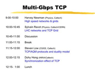
1. Multi-Gbps TCP
9:00-10:00 Harvey Newman (Physics, Caltech)
High speed networks & grids
10:00-10:45 Sylvain Ravot (Physics, Caltech/CERN)
LHC networks and TCP Grid
10:45-11:00 Discussion
11:00-11:15 Break
11:15-12:00 Steven Low (CS/EE, Caltech)
TCP/AQM protocols and duality model
12:00-12:15 Dohy Hong (INRIA/Caltech)
Synchronization effect of TCP
12:15- 1:00 Lunch

2. Multi-Gbps TCP
1:00-2:00 Fernando Paganini (EE, UCLA)
Control theory and stability of TCP/AQM
2:00-2:30 Steven Low (CS/EE, Caltech)
Stabilized Vegas (& instability of Reno/RED)
2:30-3:00 Zhikui Wang (EE, UCLA)
FAST simulations
3:00-3:15 Break
3:15-4:00 David Wei, Cheng Hu (CS, Caltech)
Some related projects and TCP kernel
4:00-4:15 Break
4:15-5:00 Discussion

3. Copyright, 1996 © Dale Carnegie & Associates,
Dualtiy Model of
TCP/AQM
Steven Low
CS & EE, Caltech
netlab.caltech.edu
2002

4. Acknowledgment
S. Athuraliya, D. Lapsley, V. Li, Q. Yin
(UMelb)
S. Adlakha (UCLA), D. Choe
(Postech/Caltech), J. Doyle (Caltech), K.
Kim (SNU/Caltech), L. Li (Caltech), F.
Paganini (UCLA), J. Wang (Caltech)
L. Peterson, L. Wang (Princeton)

5. Part I
Protocols

6. Window Flow Control
~ W packets per RTT
Lost packet detected by missing ACK
RTT
time
time
Source
Destination
1 2 W
1 2 W
1 2 W
data ACKs
1 2 W

7. Source Rate
Limit the number of packets in the network
to window W
Source rate = bps
If W too small then rate « capacity
If W too big then rate > capacity
=> congestion
RTT
MSSW ×

8. TCP Window Flow Controls
 Receiver flow control
 Avoid overloading receiver
 Set by receiver
 awnd: receiver (advertised) window
 Network flow control
 Avoid overloading network
 Set by sender
 Infer available network capacity
 cwnd: congestion window
 Set W = min (cwnd, awnd)

9. Receiver Flow Control
Receiver advertises awnd with each ACK
Window awnd
closed when data is received and ack’d
opened when data is read
Size of awnd can be the performance limit
(e.g. on a LAN)
sensible default ~16kB

10. Network Flow Control
Source calculates cwnd from indication of
network congestion
Congestion indications
Losses
Delay
Marks
Algorithms to calculate cwnd
Tahoe, Reno, Vegas, RED, REM …

11. TCP Congestion Controls
 Tahoe (Jacobson 1988)
 Slow Start
 Congestion Avoidance
 Fast Retransmit
 Reno (Jacobson 1990)
 Fast Recovery
 Vegas (Brakmo & Peterson 1994)
 New Congestion Avoidance
 RED (Floyd & Jacobson 1993)
 Probabilistic marking
 BLUE (Feng, Kandlur, Saha, Shin 1999)
 REM/PI (Athuraliya et al 2000/Hollot et al 2001)
 Clear buffer, match rate
 AVQ (Kunniyur & Srikant 2001)

12. TCP/AQM
 Tahoe (Jacobson 1988)
 Slow Start
 Congestion Avoidance
 Fast Retransmit
 Reno (Jacobson 1990)
 Fast Recovery
 Vegas (Brakmo & Peterson 1994)
 New Congestion Avoidance
 BLUE
 RED (Floyd & Jacobson 1993)
 REM/PI (Athuraliya et al 2000, Hollot et al 2001)

13. TCP Tahoe (Jacobson 1988)
SS
time
window
CA
SS: Slow Start
CA: Congestion Avoidance

14. Slow Start
Start with cwnd = 1 (slow start)
On each successful ACK increment cwnd
cwnd ← cnwd + 1
Exponential growth of cwnd
each RTT: cwnd ← 2 x cwnd
Enter CA when cwnd >= ssthresh

15. Slow Start
data packet
ACK
receiversender
1 RTT
cwnd
1
2
3
4
5
6
7
8
cwnd ← cwnd + 1 (for each ACK)

16. Congestion Avoidance
Starts when cwnd ≥ ssthresh
On each successful ACK:
cwnd ← cwnd + 1/cwnd
Linear growth of cwnd
each RTT: cwnd ← cwnd + 1

17. Congestion Avoidance
cwnd
1
2
3
1 RTT
4
data packet
ACK
cwnd ← cwnd + 1 (for each cwnd ACKS)
receiversender

18. Packet Loss
Assumption: loss indicates congestion
Packet loss detected by
Retransmission TimeOuts (RTO timer)
Duplicate ACKs (at least 3)
1 2 3 4 5 6
1 2 3
Packets
Acknowledgements
3 3
7
3

19. Fast Retransmit
Wait for a timeout is quite long
Immediately retransmits after 3 dupACKs
without waiting for timeout
Adjusts ssthresh
flightsize = min(awnd, cwnd)
ssthresh ← max(flightsize/2, 2)
Enter Slow Start (cwnd = 1)

20. Successive Timeouts
When there is a timeout, double the RTO
Keep doing so for each lost retransmission
 Exponential back-off
 Max 64 seconds1
 Max 12 restransmits1
1 - Net/3 BSD

21. Summary: Tahoe
 Basic ideas
 Gently probe network for spare capacity
 Drastically reduce rate on congestion
 Windowing: self-clocking
 Other functions: round trip time estimation, error
recovery
for every ACK {
if (W < ssthresh) then W++ (SS)
else W += 1/W (CA)
}
for every loss {
ssthresh = W/2
W = 1
}

22. TCP Reno (Jacobson 1990)
CASS
Fast retransmission/fast recovery

23. Fast recovery
 Motivation: prevent `pipe’ from emptying after
fast retransmit
 Idea: each dupACK represents a packet having
left the pipe (successfully received)
 Enter FR/FR after 3 dupACKs
 Set ssthresh ← max(flightsize/2, 2)
 Retransmit lost packet
 Set cwnd ← ssthresh + ndup (window inflation)
 Wait till W=min(awnd, cwnd) is large enough; transmit
new packet(s)
 On non-dup ACK (1 RTT later), set cwnd ← ssthresh
(window deflation)
 Enter CA

24. 9
9
4
0 0
Example: FR/FR
Fast retransmit
Retransmit on 3 dupACKs
Fast recovery
Inflate window while repairing loss to fill pipe
time
S
timeR
1 2 3 4 5 6 87
8
cwnd 8
ssthresh
1
7
4
0 0 0
Exit FR/FR
4
4
4
11
00
10 11

25. Summary: Reno
Basic ideas
Fast recovery avoids slow start
dupACKs: fast retransmit + fast recovery
Timeout: fast retransmit + slow start
slow start retransmit
congestion
avoidance FR/FR
dupACKs
timeout

26. Active queue management
Idea: provide congestion information by
probabilistically marking packets
Issues
How to measure congestion (p and G)?
How to embed congestion measure?
How to feed back congestion info?
x(t+1) = F( p(t), x(t) )
p(t+1) = G( p(t), x(t) )
Reno, Vegas
DropTail, RED, REM

27. RED (Floyd & Jacobson 1993)
 Congestion measure: average queue length
pl(t+1) = [pl(t) + xl
(t) - cl]+
 Embedding: p-linear probability function
 Feedback: dropping or ECN marking
Avg queue
marking
1

28. REM (Athuraliya & Low 2000)
 Congestion measure: price
pl(t+1) = [pl(t) + γ(αl bl(t)+ xl
(t) - cl)]+
 Embedding:
 Feedback: dropping or ECN marking

29. REM (Athuraliya & Low 2000)
 Congestion measure: price
pl(t+1) = [pl(t) + γ(αl bl(t)+ xl
(t) - cl)]+
 Embedding: exponential probability function
 Feedback: dropping or ECN marking
0 2 4 6 8 10 12 14 16 18 20
0
0.1
0.2
0.3
0.4
0.5
0.6
0.7
0.8
0.9
1
Linkcongestionmeasure
Linkmarkingprobability

30. Match rate
Clear buffer and match rate
Clear buffer
Key features
+
−++=+ )])(ˆ)(()([)1( l
l
llll ctxtbtptp αγ
)()(
11 tptp s
l −−
−⇒− φφ
Sum prices
Theorem (Paganini 2000)
Global asymptotic stability for general utility
function (in the absence of delay)

31. Active Queue Management
pl(t) G(p(t), x(t))
DropTail loss [1 - cl/xl
(t)]+
(?)
RED queue [pl(t) + xl
(t) - cl]+
Vegas delay [pl(t) + xl
(t)/cl - 1]+
REM price [pl(t) + γ(αl bl(t)+ xl
(t) - cl )]+
x(t+1) = F( p(t), x(t) )
p(t+1) = G( p(t), x(t) )
Reno, Vegas
DropTail, RED, REM

32. Congestion & performance
pl(t) G(p(t), x(t))
Reno loss [1 - cl/xl
(t)]+
(?)
Reno/RED queue [pl(t) + xl
(t) - cl]+
Reno/REM price [pl(t) + γ(αl bl(t)+ xl
(t) - cl )]+
Vegas delay [pl(t) + xl
(t)/cl - 1]+
 Decouple congestion & performance measure
 RED: `congestion’ = `bad performance’
 REM: `congestion’ = `demand exceeds supply’
But performance remains good!

33. Part II
Duality Model

34. Congestion Control
Heavy tail  Mice-elephants
Elephant
Internet
Mice
Congestion control
efficient & fair sharing small delay
queueing + propagation
CDN

35. TCP
xi(t)

36. TCP & AQM
xi(t)
pl(t)
Example congestion measure pl(t)
Loss (Reno)
Queueing delay (Vegas)

37. Outline
Protocol (Reno, Vegas, RED, REM/PI…)
Equilibrium
 Performance
 Throughput, loss, delay
 Fairness
 Utility
Dynamics
 Local stability
 Cost of stabilization
))(),(()1(
))(),(()1(
txtpGtp
txtpFtx
=+
=+

38. TCP & AQM
xi(t)
pl(t)
TCP:
 Reno
 Vegas
AQM:
 DropTail
 RED
 REM/PI
 AVQ

39. TCP & AQM
xi(t)
pl(t)
TCP:
 Reno
 Vegas
AQM:
 DropTail
 RED
 REM/PI
 AVQ

40. Model structure
F1
FN
G1
GL
Rf(s)
Rb
’
(s)
TCP Network AQM
Multi-link multi-source network
x y
q p
from F. Paganini

41. TCP Reno (Jacobson 1990)
SS
time
window
CA
SS: Slow Start
CA: Congestion Avoidance Fast retransmission/fast recovery

42. TCP Vegas (Brakmo & Peterson 1994)
SS
time
window
CA
 Converges, no retransmission
 … provided buffer is large enough

43. queue size
for every RTT
{ if W/RTTmin – W/RTT < α then W ++
if W/RTTmin – W/RTT > α then W -- }
for every loss
W := W/2
Vegas model
pl(t+1) = [pl(t) + yl (t)/cl - 1]+
Gl:
( )



<+=+ iiii
i
ii dtqtx
D
txtx α)()(if
1
)(1 2
( ) else)(1 txtx ss =+
Fi:
( )



>−=+ iiii
i
ii dtqtx
D
txtx α)()(if
1
)(1 2

44. Vegas model
F1
FN
G1
GL
Rf(s)
Rb
’
(s)
TCP Network AQM
x y
q p
+






−+= 1
)(
)(
l
l
ll
c
ty
tpG
( ))()(sgn
))((
1
)( 2
tqtxd
tqd
txF iiii
ii
ii −
+
+= α

45. Overview
Protocol (Reno, Vegas, RED, REM/PI…)
Equilibrium
 Performance
 Throughput, loss, delay
 Fairness
 Utility
Dynamics
 Local stability
 Cost of stabilization
))(),(()1(
))(),(()1(
txtpGtp
txtpFtx
=+
=+

46. Model
c1 c2
 Network
 Links l of capacities cl
Sources i
L(s) - links used by source i
Ui(xi) - utility if source rate = xi
x1
x2
x3
121 cxx ≤+ 231 cxx ≤+

47. Primal problem
Llcy
xU
ll
i
ii
xi
∈∀≤
∑≥
,subject to
)(max
0
Assumptions
Strictly concave increasing Ui
 Unique optimal rates xi exist
 Direct solution impractical

48. Related Work
 Formulation
 Kelly 1997
 Penalty function approach
 Kelly, Maulloo & Tan 1998
 Kunniyur & Srikant 2000
 Duality approach
 Low & Lapsley 1999
 Athuraliya & Low 2000
 Extensions
 Mo & Walrand 2000
 La & Anantharam 2000
 Dynamics
 Johari & Tan 2000, Massoulie 2000, Vinnicombe 2000, …
 Hollot, Misra, Towsley & Gong 2001
 Paganini 2000, Paganini, Doyle, Low 2001, …

49. Duality Approach
))(),(()1(
))(),(()1(
txtpGtp
txtpFtx
=+
=+
Primal-dual algorithm:






−+=
∈∀≤
∑∑
∑
≥≥
≥
)()(max)(min
,subject to)(max
00
0
:Dual
:Primal
l
l
l
l
s
ss
xp
l
l
s
ss
x
xcpxUpD
LlcxxU
s
s

50. Duality Model of TCP
))(),(()1(
))(),(()1(
txtpGtp
txtpFtx
=+
=+
Primal-dual algorithm:
Reno, Vegas
DropTail, RED, REM
 Source algorithm iterates on rates
 Link algorithm iterates on prices
 With different utility functions

51. Duality Model of TCP
))(),(()1(
))(),(()1(
txtpGtp
txtpFtx
=+
=+
Primal-dual algorithm:
Reno, Vegas
DropTail, RED, REM
(x*,p*) primal-dual optimal if and only if
0ifequalitywith **
>≤ lll pcy

52. Duality Model of TCP
))(),(()1(
))(),(()1(
txtpGtp
txtpFtx
=+
=+
Primal-dual algorithm:
Reno, Vegas
DropTail, RED, REM
Any link algorithm that stabilizes queue
 generates Lagrange multipliers
 solves dual problem

53. Gradient algorithm
 Gradient algorithm
))(()1(:source 1'
tqUtx iii
−
=+
+
−+=+ )])(()([)1(:link lllll ctytptp γ
Theorem (Low & Lapsley ’99)
Converge to optimal rates in distributed
asynchronous environment

54. Gradient algorithm
 Gradient algorithm
))(()1(:source 1'
tqUtx iii
−
=+
+
−+=+ )])(()([)1(:link lllll ctytptp γ
 Vegas: approximate gradient algorithm
( ))()(sgn
))((
1
)( 2
txtx
tqd
txF ii
ii
ii −
+
+=
))((1'
tqU ii
−

55. Summary: equilibrium
Llcx
xU
l
l
s
ss
xs
∈∀≤
∑≥
,subject to
)(max0
 Flow control problem
 TCP/AQM
 Maximize aggregate source utility
 With different utility functions
 Primal-dual algorithm
))(),(()1(
))(),(()1(
txtpGtp
txtpFtx
=+
=+ Reno, Vegas
DropTail, RED, REM

56. Implications
Performance
Rate, delay, queue, loss
Fairness
Utility function
Persistent congestion

57. Performance
Delay
Congestion measures: end to end queueing
delay
Sets rate
Equilibrium condition: Little’s Law
Loss
No loss if converge (with sufficient buffer)
Otherwise: revert to Reno (loss unavoidable)
)(
)(
tq
d
tx
s
s
ss α=

58. Vegas Utility
iiiii xdxU log)( α=
Equilibrium (x, p) = (F, G)
Proportional fairness

59. Validation (L. Wang, Princeton)
Source 1 Source 3 Source 5
RTT (ms) 17.1 (17) 21.9 (22) 41.9 (42)
Rate (pkts/s) 1205 (1200) 1228 (1200) 1161 (1200)
Window (pkts) 20.5 (20.4) 27 (26.4) 49.8 (50.4)
Avg backlog (pkts) 9.8 (10)
NS-2 simulation, single link, capacity = 6 pkts/ms
5 sources with different propagation delays, αs = 2 pkts/RTT
meausred theory

60. Persistent congestion
 Vegas exploits buffer process to compute prices
(queueing delays)
 Persistent congestion due to
 Coupling of buffer & price
 Error in propagation delay estimation
 Consequences
 Excessive backlog
 Unfairness to older sources
Theorem (Low, Peterson, Wang ’02)
A relative error of εs in propagation delay estimation
distorts the utility function to
sssssssss xdxdxU εαε ++= log)1()(ˆ

61. Validation (L. Wang, Princeton)
 Single link, capacity = 6 pkt/ms, αs = 2 pkts/ms, ds = 10 ms
 With finite buffer: Vegas reverts to Reno
Without estimation error With estimation error

62. Validation (L. Wang, Princeton)
Source rates (pkts/ms)
# src1 src2 src3 src4 src5
1 5.98 (6)
2 2.05 (2) 3.92 (4)
3 0.96 (0.94) 1.46 (1.49) 3.54 (3.57)
4 0.51 (0.50) 0.72 (0.73) 1.34 (1.35) 3.38 (3.39)
5 0.29 (0.29) 0.40 (0.40) 0.68 (0.67) 1.30 (1.30) 3.28 (3.34)
# queue (pkts) baseRTT (ms)
1 19.8 (20) 10.18 (10.18)
2 59.0 (60) 13.36 (13.51)
3 127.3 (127) 20.17 (20.28)
4 237.5 (238) 31.50 (31.50)
5 416.3 (416) 49.86 (49.80)

63. Vegas/REM
Vegas/REM Vegas
peak = 43 pkts
utilization : 90% - 96%

64. Outline
Protocol (Reno, Vegas, RED, REM/PI…)
Equilibrium
 Performance
 Throughput, loss, delay
 Fairness
 Utility
Dynamics
 Local stability
 Cost of stabilization
))(),(()1(
))(),(()1(
txtpGtp
txtpFtx
=+
=+

65. Vegas model
F1
FN
G1
GL
Rf(s)
Rb
’
(s)
TCP Network AQM
x y
q p
+






−+= 1
)(
)(
l
l
ll
c
ty
tpG
( ))()(sgn
))((
1
)( 2
tqtxd
tqd
txF iiii
ii
ii −
+
+= α

66. Vegas model
F1
FN
G1
GL
Rf(s)
Rb
’
(s)
TCP Network AQM
x y
q p
[ ] lieR lis
lif linkusessourceifτ

−
=
[ ] lieR lis
lib linkusessourceifτ

−
=

67. Approximate model
( )ii
ii
d
tqtx
i
tT
tx α
)()(
2
1sgn
)(
1
)( −=

68. Approximate model
( )ii
ii
d
tqtx
i
tT
tx α
)()(
2
1sgn
)(
1
)( −=
( )ii
ii
d
tqtx
i
tT
tx αη
π
)()(1-
2
1tan
)(
12
)( −=

69. Linearized model
i
ii
i
i
i
i q
asT
a
q
x
x ∂
+
−=∂ l
l
l y
c
p ∂−=∂
γ

F1
FN
G1
GL
Rf(s)
Rb
’
(s)
TCP Network AQM
x y
q p
12
ii
i
Tx
a
π
η
−= γ controls equilibrium delay

70. Stability
Cannot be satisfied with >1 bottleneck link!
Theorem (Choe & Low, ‘02)
Locally asymptotically stable if
c
c
i
i
a
a
ω
ωsin
mintimetriproud
delayqueueinglink
> > 0.63

71. Stabilized Vegas
( ))(1tan
)(
12
)( )()(1-
2
tq
tT
tx iid
tqtx
i ii
ii
 κη
π α −−=
( )ii
ii
d
tqtx
i
tT
tx αη
π
)()(1-
2
1tan
)(
12
)( −=

72. Linearized model
i
ii
i
i
i
i q
asT
a
q
x
x ∂
+
−=∂ l
l
l y
c
p ∂−=∂
γ

F1
FN
G1
GL
Rf(s)
Rb
’
(s)
TCP Network AQM
x y
q p
γ controls equilibrium delay

73. Linearized model
i
ii
i
ii q
as
as
bx ∂
+
+
−=∂
µ
 l
l
l y
c
p ∂−=∂
γ

F1
FN
G1
GL
Rf(s)
Rb
’
(s)
TCP Network AQM
x y
q p
γ controls equilibrium delaychoose ai = a, αi = µ

74. Stability
Theorem (Choe & Low, ‘02)
Locally asymptotically stable if
),(
queueingtripround
timetripround
µaσM <
example
 LHS < 10*10 = 100
 a = 0.1, µ = 0.015  σ (a,µ) = 120

75. Stability
Theorem (Choe & Low, ‘02)
Locally asymptotically stable if
),(
queueingtripround
timetripround
µaσM <
Application
 Stabilized TCP with current routers
 Queueing delay as congestion measure has the right scaling
 Incremental deployment with ECN

76. Papers
 A duality model of TCP flow controls (ITC, Sept 2000)
 Optimization flow control, I: basic algorithm &
convergence (ToN, 7(6), Dec 1999)
 Understanding Vegas: a duality model (J. ACM, 2002)
 Scalable laws for stable network congestion
control (CDC, 2001)
 REM: active queue management (Network, May/June 2001)
netlab.caltech.edu

77. Backup slides

78. Dynamics
Small effect on queue
AIMD
Mice traffic
Heterogeneity
Big effect on queue
Stability!

79. Stable: 20ms delay
0 1000 2000 3000 4000 5000 6000 7000 8000 9000 10000
0
10
20
30
40
50
60
70
Window
time (ms)
Window(pkts)
individual window
Window
Ns-2 simulations, 50 identical FTP sources, single link 9 pkts/ms, RED marking

80. 0 1000 2000 3000 4000 5000 6000 7000 8000 9000 10000
0
100
200
300
400
500
600
700
800
Instantaneous queue
time (ms)
Instantaneousqueue(pkts)
Queue
Stable: 20ms delay
0 1000 2000 3000 4000 5000 6000 7000 8000 9000 10000
0
10
20
30
40
50
60
70
Window
time (ms)
Window(pkts)
individual window
0 1000 2000 3000 4000 5000 6000 7000 8000 9000 10000
0
10
20
30
40
50
60
70
Window
time (ms)
Window(pkts)
individual window
average window
Window
Ns-2 simulations, 50 identical FTP sources, single link 9 pkts/ms, RED marking

81. 0 1000 2000 3000 4000 5000 6000 7000 8000 9000 10000
0
10
20
30
40
50
60
70
Window
time (10ms)
Window(pkts)
individual window
Unstable: 200ms delay
Window
Ns-2 simulations, 50 identical FTP sources, single link 9 pkts/ms, RED marking

82. 0 1000 2000 3000 4000 5000 6000 7000 8000 9000 10000
0
10
20
30
40
50
60
70
Window
time (10ms)
Window(pkts)
individual window
0 1000 2000 3000 4000 5000 6000 7000 8000 9000 10000
0
10
20
30
40
50
60
70
Window
time (10ms)
Window(pkts)
individual window
average window
Unstable: 200ms delay
0 1000 2000 3000 4000 5000 6000 7000 8000 9000 10000
0
100
200
300
400
500
600
700
800
Instantaneous queue
time (10ms)
Instantaneousqueue(pkts)
QueueWindow
Ns-2 simulations, 50 identical FTP sources, single link 9 pkts/ms, RED marking

83. Other effects on queue
0 1000 2000 3000 4000 5000 6000 7000 8000 9000 10000
0
100
200
300
400
500
600
700
800
Instantaneous queue
time (ms)
Instantaneousqueue(pkts)
0 1000 2000 3000 4000 5000 6000 7000 8000 9000 10000
0
100
200
300
400
500
600
700
800
Instantaneous queue
time (10ms)
Instantaneousqueue(pkts)
20ms
200ms
0 10 20 30 40 50 60 70 80 90 100
0
100
200
300
400
500
600
700
800
Instantaneous queue (50% noise)
time (sec)
instantaneousqueue(pkts)
50% noise
0 10 20 30 40 50 60 70 80 90 100
0
100
200
300
400
500
600
700
800
Instantaneous queue (50% noise)
time (sec)
instantaneousqueue(pkts)
50% noise
0 10 20 30 40 50 60 70 80 90 100
0
100
200
300
400
500
600
700
800
time (sec)
Instantaneous queue (pkts)
instantaneousqueue(pkts)
avg delay 16ms
0 10 20 30 40 50 60 70 80 90 100
0
100
200
300
400
500
600
700
800
time (sec)
Instantaneous queue (pkts)
instantaneousqueue(pkts)
avg delay 208ms

84. Effect of instability
Larger jitters in throughput
Lower utilization
20 40 60 80 100 120 140 160 180 200
0
20
40
60
80
100
120
140
160
delay (ms)
window
Mean and variance of individual window
mean
variance
No noise

85. Linearized system
F1
FN
G1
GL
Rf(s)
Rb
’
(s)
TCP Network AQM
x y
q p
( ) ))(),(),((
~
:)(),( tytptzGtytpG lllllll =
( ) )(
2
)())(1(
)()(),(
2
2
tq
txtq
txtxtqF i
i
i
i
iiii −
−
+=
τ

86. Linearized system
F1
FN
G1
GL
Rf(s)
Rb
’
(s)
x y
q p
s
n
s
n
ni ii
i
n
e
e
x
c
scs
c
wpsp
sL τ
βτ
τ
α
ρα
ττ
−
−
⋅
+
⋅
+
⋅
+
=
∑
∑ 1
1
)(
1
)( ***
TCP RED queue delay

87. Stability condition
Theorem: TCP/RED stable if
222
2
3
33
)1(4
)1
)(
2 ππβ
βπ
τ
τρ
−+
≤+⋅
-(
Nc
N
c
ω=0
∞=ω
TCP:
 Small τ
 Small c
 Large N
RED:
 Small ρ
 Large delay

88. Validation
50 55 60 65 70 75 80 85 90 95 100
50
55
60
65
70
75
80
85
90
95
100
Round trip propagation delay at critical frequency (ms)
delay (NS)
delay(model)
0 0.5 1 1.5 2 2.5 3 3.5 4 4.5 5
0
0.5
1
1.5
2
2.5
3
3.5
4
4.5
5
Critical frequency (Hz)
frequency (NS)
frequency(model) dynamic-link model
30 data points

89. 0 0.5 1 1.5 2 2.5 3 3.5 4 4.5 5
0
0.5
1
1.5
2
2.5
3
3.5
4
4.5
5
Critical frequency (Hz)
frequency (NS)
frequency(model) dynamic-link model
30 data points
Validation
50 55 60 65 70 75 80 85 90 95 100
50
55
60
65
70
75
80
85
90
95
100
Round trip propagation delay at critical frequency (ms)
delay (NS)
delay(model)
0 0.5 1 1.5 2 2.5 3 3.5 4 4.5 5
0
0.5
1
1.5
2
2.5
3
3.5
4
4.5
5
Critical frequency (Hz)
frequency (NS)
frequency(model) dynamic-link model
static-link model
30 data points

90. Stability region
8 9 10 11 12 13 14 15
50
55
60
65
70
75
80
85
90
95
100
Round trip propagation delay at critical frequency
capacity (pkts/ms)
delay(ms)
N=40
N=30
N=20
N=20 N=60
Unstable for
 Large delay
 Large capacity
 Small load

91. Role of AQM
(Sufficient) stability condition
-1
});({co θωHK ⋅

92. Role of AQM
(Sufficient) stability condition
-1
});({co θωHK ⋅
TCP:
N
c
2
22
τ
**
wpj
e j
+
−
ω
ω
AQM: scale down K & shape H

93. Role of AQM
});({co θωHK ⋅
TCP:
N
c
2
22
τ
**
wpj
e j
+
−
ω
ω
RED:
β
ταρ
−1
c
ταωω
θ
cj
e j
+
⋅
−
1
REM/PI:
β
τ
−1
2a
ω
τω
ω
θ
j
aaje j
21 /+
⋅
−
Queue dynamics (windowing)
Problem!!

94. Role of AQM
To stabilize a given TCP Fi with least cost
),(subject to
)()()()(min
0)(
pxFx
dttRptptxQtx TT
p
=
+∫
∞
⋅

 Linearized F, single link, identical sources

Any AQM solves
optimal control with appropriate Q and R
))()()(()( 321
*
tyktyktbktp  ++−=
))()()(()( 321 tyktyktbktp  ++−=

95. Role of AQM
To stabilize a given TCP Fi with least cost
),(subject to
)()()()(min
0)(
pxFx
dttRptptxQtx TT
p
=
+∫
∞
⋅

 Linearized F, single link, identical sources


))()()(()( 321
*
tyktyktbktp  ++−=
k1=0
Nonzero buffer
k3=0
Slower decay