SlideShare une entreprise Scribd logo
1  sur  10
ecomputernotes.com – Data Structures
Lecture No. 13
___________________________________________________________________
Data Structures
Lecture No. 13
In the previous lecture, we had written and demonstrated the use of C++ code of
insert routine for a tree through an example. We also saw how a new node is inserted
into a binary tree. If the to-be-inserted number (node) is already in the tree i.e. it
matches a number already present in the tree, we display a message that the number is
already in the tree. In the last lecture, the advantages of the tree data structure vis-à-vis
linked list data structure were also discussed. In a linked list, a programmer has to
search the whole list to find out a duplicate of a number to be inserted. It is very
tedious job as the number of stored items in a linked list is very large. But in case of
tree data structure, we get a dynamic structure in which any number of items as long as
memory is available, can be stored. By using tree data structure, the search operation
can be carried out very fast. Now we will see how the use of binary tree can help in
searching the duplicate number in a very fast manner.
Cost of Search
Consider the previous example where we inserted the number 17 in the tree. We
executed a while loop in the insert method and carried out a comparison in while loop.
If the comparison is true, it will reflect that in this case, the number in the node where
the pointer p is pointing is not equal to 17 and also q is not NULL. Then we move p
actually q to the left or right side. This means that if the condition of the while loop is
true then we go one level down in the tree. Thus we can understand it easily that if
there is a tree of 6 levels, the while loop will execute maximum 6 times. We conclude
from it that in a given binary tree of depth d, the maximum number of executions of the
while loop will be equal to d. The code after the while loop will do the process
depending upon the result of the while loop. It will insert the new number or display a
message if the number was already there in the tree.
Now suppose we have another method find. This method does not insert a new
number in the tree. Rather, it traverses a tree to find if a given number is already
present in the tree or not. The tree which the find method traverses was made in such
an order that all the numbers less than the number at the root are in the left sub-tree of
the root while the right sub-tree of the root contains the numbers greater than the
number at the root. Now the find method takes a number x and searches out its
duplicate in the given tree. The find method will return true if x is present in the tree.
Otherwise, it will return false. This find method does the same process that a part of
the insert method performs. The difference is that the insert method checks for a
duplicate number before putting a number in the tree whereas the find method only
finds a number in the tree. Here in the find method, the while loop is also executed at
maximum equal to the number of levels of the tree. We do a comparison at each level
of the tree until either x is found or q becomes NULL. The loop terminates in case, the
number is found or it executes to its maximum number, i.e. equal to the number of
levels of the tree.
Page 1 of 10
ecomputernotes.com – Data Structures
Lecture No. 13
___________________________________________________________________
In the discussion on binary tree, we talked about the level and number of nodes of a
binary tree. It was witnessed that if we have a complete binary tree with n numbers of
nodes, the depth d of the tree can be found by the following equation:
d = log2 (n + 1) – 1
Suppose we have a complete binary tree in which there are 100,000 nodes, then its
depth d will be calculated in the following fashion.
d = log2 (100000 + 1) – 1 = log2 (100001) – 1= 20
The statement shows that if there are 100,000 unique numbers (nodes) stored in a
complete binary tree, the tree will have 20 levels. Now if we want to find a number x in
this tree (in other words, the number is not in the tree), we have to make maximum 20
comparisons i.e. one comparison at each level. Now we can understand the benefit of
tree as compared to the linked list. If we have a linked list of 100,000 numbers, then
there may be 100,000 comparisons (supposing the number is not there) to find a
number x in the list.
Thus in a tree, the search is very fast as compared to the linked list. If the tree is
complete binary or near-to-complete, searching through 100,000 numbers will require
a maximum of 20 comparisons or in general, approximately log2(n). Whereas in a
linked list, the comparisons required could be a maximum of n.
Tree with the linked structure, is not a difficult data structure. We have used it to
allocate memory, link and set pointers to it. It is not much difficult process. In a tree,
we link the nodes in such a way that it does not remain a linear structure. If instead of
100,000, we have 1 million or 10 million or say, 1 billion numbers and want to build a
complete binary tree of these numbers, the depth (number of levels) of the tree will be
log2 of these numbers. The log2 of these numbers will be a small number, suppose 25,
30 or 40. Thus we see that the number of level does not increase in such a ratio as the
number of nodes increase. So we can search a number x in a complete binary tree of 1
billion nodes only in 30-40 comparisons. As the linked list of such a large number
grows large, the search of a number in such a case will also get time consuming
process. The usage of memory space does not cause any effect in the linked list and
tree data structures. We use the memory dynamically in both structures. However,
time is a major factor. Suppose one comparison takes one micro second, then one
billion seconds are required to find a number from a linked list (we are supposing the
worst case of search where traversing of the whole list may be needed). This time will
be in hours. On the other hand, in case of building a complete binary tree of these one
billion numbers, we have to make 30-40 comparisons (as the levels of the tree will be
30-40), taking only 30-40 microseconds. We can clearly see the difference between
hours and microseconds. Thus it is better to prefer the process of building a tree of the
data to storing it in a linked list to make the search process faster.
Binary Search Tree
While discussing the search procedure, the tree for search was built in a specific order.
The order was such that on the addition of a number in the tree, we compare it with a
node. If it is less than this, it can be added to the left sub-tree of the node. Otherwise, it
will be added on the right sub-tree. This way, the tree built by us has numbers less than
the root in the left sub-tree and the numbers greater than the root in the right sub-tree.
Page 2 of 10
14
4 15
ecomputernotes.com – Data Structures
Lecture No. 13
___________________________________________________________________
A binary tree with such a property that items in the left sub-tree are smaller than the
root and items in the right sub-tree are larger than the root is called a binary search
tree (BST). The searching and sorting operations are very common in computer
science. We will be discussing them many times during this course. In most of the
cases, we sort the data before a search operation. The building process of a binary
search tree is actually a process of storing the data in a sorted form. The BST has
many variations, which will be discussed later. The BST and its variations play an
important role in searching algorithms. As data in a BST is in an order, it may also be
termed as ordered tree.
Traversing a Binary Tree
Now let’s discuss the ways to print the numbers present in a BST. In a linked list, the
printing of stored values is easy. It is due to the fact that we know wherefrom, a
programmer needs to start and where the next element is. Equally is true about printing
of the elements in an array. We execute a for loop starting from the first element (i.e.
index 0) to the last element of the array. Now let’s see how we can traverse a tree to
print (display) the numbers (or any data items) of the tree.
We can explain this process with the help of the following example in which we
traverse a binary search tree. Suppose there are three nodes tree with three numbers
stored in it as shown below.
Fig 13.1: A three node binary tree
Here we see that the root node has the number 14. The left sub-tree has only one node
i.e. number 4. Similarly the right sub-tree consists of a single node with the number 15.
If we apply the permutations combinations on these three nodes to print them, there
may be the following six possibilities.
1: (4, 14, 15)
2: (14, 4, 15)
3: (15, 4, 14)
4: (4, 15, 14)
5: (14, 15, 4)
6: (15, 14, 4)
Page 3 of 10
ecomputernotes.com – Data Structures
Lecture No. 13
___________________________________________________________________
Look at these six combinations of printing the nodes of the tree. In the first
combination, the order of printing the nodes is 4-14-15. It means that left subtree-root-
right subtree. In the second combination the order is root-left subtree-right subtree. In
the third combination, the order of printing the nodes is right subtree-root-left subtree.
The fourth combination has left subtree-right subtree-root. The fifth combination has
the order root-rigth subtree- left subtree. Finally the sixth combination has the order of
printing the nodes right subtree-root-left subtree. These six possibilities are for the
three nodes only. If we have a tree having a large number of nodes, then there may
increase number of permutations for printing the nodes.
Let’s see the general procedure of traversing a binary tree. We know by definition that
a binary tree consists of three sets i.e. root, left subtree and right subtree. The
following figure depicts a general binary tree.
Fig 13.2: A generic binary tree
In this figure, we label the root node with N. The left subtree in the figure is in a
triangle labeled as L. This left subtree may consist of any number of nodes. Similarly
the right subtree is enclosed in a triangle having the label R. This triangle of right
subtree may contain any number of nodes. Following are the six permutations, which
we have made for the three nodes previously. To generalize these permutations, we
use N, L and R as abbreviations for root, left subtree and right subtree respectively.
1: (L, N, R)
2: (N, L, R)
3: (R, L, N)
4: (L, R, N)
5: (N, R, L)
6: (R, N, L)
In these permutations, the left and right subtree are not single nodes. These may
consist of several nodes. Thus where we see L in the permutations, it means traversing
the left subtree. Similarly R means traversing the right subtree. In the previous tree of
three nodes, these left and right subtrees are of single nodes. However, they can
consist of any number of nodes. We select the following three permutations from the
Page 4 of 10
node
left
subtre
e
right
subtree
N
L R
ecomputernotes.com – Data Structures
Lecture No. 13
___________________________________________________________________
above six. The first of these three is (N, L, R), also called as preorder traversal. The
second permutation is (L, N, R) which we called inorder traversal. Finally the third
permutation, also termed as postorder traversal is (L, R, N). Now we will discuss these
preorder, inorder and postorder traversal in detail besides having a look on their
working. We will also see the order in which the numbers in the tree are displayed by
these traversing methods.
C++ code
Let’s write the C++ code for it. Following is the code of the preorder method.
void preorder(TreeNode<int>* treeNode)
{
if( treeNode != NULL )
{
cout << *(treeNode->getInfo())<<" ";
preorder(treeNode->getLeft());
preorder(treeNode->getRight());
}
}
In the arguments, there is a pointer to a TreeNode. We may start from any node and
the pointer of the node will be provided as argument to the preorder method. In this
method, first of all we check whether the pointer provided is NULL or not. If it is not
NULL, we print the information stored in that node with the help of the getInfo()
method. Then we call the getLeft() method that returns a pointer of left node, which
may be a complete subtree. With the help of this method, we get the root of that
subtree. We call the preorder method again passing that pointer. When we return from
that, the preorder method is called for the right node. Let’s see what is happening in
this method. We are calling the preorder method within the preorder method. This is
actually a recursive call. Recursion is supported in C++ and other languages.
Recursion means that a function can call itself. We may want to know why we are
doing this recursive call. We will see some more examples in this regard and
understand the benefits of recursive calls. For the time being, just think that we are
provided with a tree with a root pointer. In the preorder, we have to print the value of
the root node. Don’t think that you are in the preorder method. Rather keep in mind
that you have a preorder function. Suppose you want to print out the left subtree in the
preorder way. For this purpose, we will call the preorder function. When we come
back, the right subtree will be printed. In the right subtree, we will again call the
preorder function that will print the information. Then call the preorder function for
the left subtree and after that its right subtree. It will be difficult if you try to do this
incursion in the mind. Write the code and execute it. You must be knowing that the
definition of the binary tree is recursive. We have a node and left and right subtrees.
What is left subtree? It is also a node with a left subtree and right subtree. We have
shown you how the left subtree and right subtree are combined to become a tree. The
definition of tree is itself recursive. You have already seen the recursive functions. You
have seen the factorial example. What is factorial of N? It is N multiplied by N-1
factorial. What is N-1 factorial? N-1 factorial is N-1 multiplied by N-2 factorial. This is
the recursive definition. For having an answer, it is good to calculate the factorial of
Page 5 of 10
ecomputernotes.com – Data Structures
Lecture No. 13
___________________________________________________________________
one less number till the time you reach at the number 2. You will see these recursions
or recursive relations here and also in mathematic courses. In the course of discrete
mathematics, recursion method is used. Here we are talking about the recursive calls.
We will now see an example to understand how this recursive call works and how can
we traverse the tree using the recursion. One of the benefits of recursion that it prints
out the information of all the nodes without caring for the size of the tree. If the tree
has one lakh nodes, this simple four lines routine will print all the nodes. When
compared with the array printing, we have a simple loop there. In the link list also, we
have a small loop that executes till the time we have a next pointer as NULL. For tree,
we use recursive calls to print it.
Here is the code of the inorder function.
void inorder(TreeNode<int>* treeNode)
{
if( treeNode != NULL )
{
inorder(treeNode->getLeft());
cout << *(treeNode->getInfo())<<" ";
inorder(treeNode->getRight());
}
}
The argument is the same as in the preorder i.e. a pointer to the TreeNode. If this node
is not NULL, we call getLeft() to get the left node and call the inorder function. We
did not print the node first here. In the inorder method, there is no need to print the
root tree first of all. We start with the left tree. After completely traversing the
complete left tree, we print the value of the node. In the end, we traverse the right
subtree in recursion.
Hopefully, you have now a fair knowledge about the postorder mechanism too. Here is
the code of the postorder method.
void postorder(TreeNode<int>* treeNode)
{
if( treeNode != NULL )
{
postorder(treeNode->getLeft());
postorder(treeNode->getRight());
cout << *(treeNode->getInfo())<<" ";
}
}
In the postorder, the input argument is a pointer to the TreeNode. If the node is not
NULL, we traverse the left tree first. After that we will traverse the right tree and print
the node value from where we started.
Page 6 of 10
Fig 13.3: Preorder: 14 4 3 9 7 5 15 18 16 17
20
14
154
9
7
183
5
16 20
17
ecomputernotes.com – Data Structures
Lecture No. 13
___________________________________________________________________
As all of these above routines are function so we will call them as:
cout << "inorder: ";
preorder( root);
cout << "inorder: ";
inorder( root );
cout << "postorder: ";
postorder( root );
Here the root represents the root node of the tree. The size of the tree does not matter
as the complete tree will be printed in preorder, inorder and postorder. Let’s discuss
an example to see the working of these routines.
Example
Let’s have a look on the following tree.
This is the same tree we have been using previously. Here we want to traverse the tree.
In the bottom of the figure, the numbers are printed with the help of preorder method.
These numbers are as 14 4 3 9 7 5 15 18 16 17 20. Now take these numbers and
traverse the tree. In the preorder method, we print the root, followed by traversing of
the left subtree and the right subtree respectively. As the value of the root node is 14,
so it will be printed first of all. After printing the value of the root node, we call the
preorder for the left node which is 4. Forget the node 14 as the root is 4 now. So the
value 4 is printed and we call the preorder again with the left sub tree i.e. the node with
value 3. Now the root is the node with value 3. We will print its value before going to
its left. The left side of node with value 3 is NULL. Preorder will be called if condition
Page 7 of 10
Fig 13.4: Inorder: 3 4 5 7 9 14 15 16 17 18
20
14
154
9
7
183
5
16 20
17
ecomputernotes.com – Data Structures
Lecture No. 13
___________________________________________________________________
is false. In this case, no action will be taken. Now the preorder of the left subtree is
finished. As the right subtree of this node is also NULL, so there is no need of any
action. Now the left subtree of the node with value 4 is complete. The method
preorder will be called for the right subtree of the node with value 4. So we call the
preorder with the right node of the node with value 4. Here, the root is the node with
value 9 that is printed. We will call its left subtree where the node value is 7. It will be
followed by its left subtree i.e. node 5 which will be printed.
In the preorder method, we take the root i.e. 14 in this case. Its value is printed,
followed by its left subtree and so on. This activity takes us to the extreme left node.
Then we back track and print the right subtrees.
Let’s try to understand the inorder method from the following statement.
When we call the inorder function, the numbers will be printed as 3 4 5 7 9 14 15 16
17 18 20. You might have noted that these numbers are in sorted order. When we
build the tree, there was no need of sorting the numbers. But here we have the sorted
numbers in the inorder method. While inserting a new node, we compare it with the
existing ones and place the new node on the left or right side. So during the process of
running the inorder on the binary tree, a programmer gets the numbers sorted.
Therefore we have a sorting mechanism. If we are given some number, it will not be
difficult to get them sorted. This is a new sorting algorithm for you. It is very simple.
Just make BST with these numbers and run the inorder traversal. The numbers
obtained from the inorder traversal are sorted.
In the inorder method, we do not print the value of node first. We go to traverse its
left subtree. When we come back from the left subtree and print the value of this node.
Afterwards, we go to the right subtree. Now consider the above tree of figure 13.4. If
we start from number 14, it will not be printed. Then we will go to the left subtree.
The left subtree is itself a tree. The number 4 is its root. Now being at the node 4, we
again look if there is any left subtree of this node. If it has a left subtree, we will not
Page 8 of 10
ecomputernotes.com – Data Structures
Lecture No. 13
___________________________________________________________________
print 4 and call the inorder method on its left subtree. As there is a left subtree of 4
that consists a single node i.e. 3, we go to that node. Now we call the inorder of node
3 to see if there is a subtree of it. As there is no left subtree of 3, the if statement that
checks if the node is not NULL will become false. Here the recursive calls will not be
executed. We will come back from the call and print the number 3. Thus the first
number that is printed in the inorder traversal is 3. After printing 3, we go to its right
subtree that is also NULL. So we come back to node 3. Now as we have traversed the
left and right subtrees of 3 which itself is a left subtree of 4, thus we have traversed the
left subtree of 4. Now we print the value 4 and go to the right subtree of 4. We come
at node 9. Before printing 9 we go to its left subtree that leads us to node 7. In this
subtree with root 7, we will not print 7. Now we will go to its left subtree which is
node 5. We look for the left subtree of 5 which is NULL. Now we print the value 5.
Thus, we have so far printed the numbers 3, 4 and 5. Now we come back to 7. After
traversing its left subtree, we print the number 7. The right subtree of 7 is NULL. Thus
finally, we have traversed the whole tree whose root is 7. It is a left subtree of 9. Now,
we will come back to 9 and print it (as its left subtree has been traversed). The right
subtree of 9 is NULL. So there is no need to traverse it. Thus the whole tree having 9
as its root has been traversed. So we come back to the root 4, the right subtree of
which is the tree with root 9. Resultantly, the left and right subtree of 4 have been
traversed now. Thus we have printed the numbers 3, 4, 5, 7 and 9. Now from here
(i.e. node 4) we go to the node 14 whose left subtree has been traversed. Now we
print 14 and go to its right subtree. The right subtree of 14 has 15 as the root. From
here, we repeat the same process earlier carried out in case of the left subtree of 14. As
a result of this process, the numbers 15, 16, 17, 18 and 20 are printed. Thus we get the
numbers stored in the tree in a sorted order. And we get the numbers printed as 3, 4, 5,
7, 9, 14, 15, 16, 17, 18, 20. This sorted order is only in the inorder traversal.
When we apply the post order traversal on the same tree, the numbers we get are not
in sorted order. The numbers got through postorder traversal are in the following
order:
3 5 7 9 4 17 16 20 18 15 14
We see that these are not in a sorted order.
We know that every function has a signature. There is return type, function name and
its parameter list in the signature of a function. Then there comes the body of the
function. In the body of a function, there may be local variables and calls to some other
functions. Now if a statement in the body of a function is calling the same function in
which it exists, it will be termed as a recursive call. For example if a statement in
function A is calling the function A, it is a recursive call and the process is called
recursion.
Now let’s see how recursion is carried out. We know that the function calls are
implemented through stacks at run time. Let’s see what happens when there is a
recursive call. In a recursive call that means calling a function itself makes no
difference as far as the call stack is concerned. It is the same as a function F calls a
function G, only with the difference that now function F is calling to function F instead
of G. The following figure shows the stack layout when function F calls function F
recursively.
Page 9 of 10
ecomputernotes.com – Data Structures
Lecture No. 13
___________________________________________________________________
Fig 13.5
When F is called first time, the parameters, local variables and its return address are
put in a stack, as some function has called it. Now when F calls F, the stack will
increase the parameters, local variables and return address of F comes in the stack
again. It is the second call to F. After coming back from this second call, we go to the
state of first call of F. The stack becomes as it was at first call. In the next lecture, we
will see the functionality of recursive calls by an example.
Exercise
Please find out the preorder, inorder and postorder traversal of the tree given below:
Page 10 of 10
Parameters(F)
Local variables(F)
Return address(F)
Parameters(F)
Parameters(F)
Return address(F)
Parameters(F)
Local variables(F)
Return address(F)
Parameters(F)
Local variables(F)
Return address(F)
During execution of F After callAt point of call
sp
sp
sp
Local variables(F)
Fig 13.6
40
5014
19
17
8010
15
60 200
70
12
11
16
45
46
55
42
44

Contenu connexe

Tendances

Binary Search Tree (BST)
Binary Search Tree (BST)Binary Search Tree (BST)
Binary Search Tree (BST)M Sajid R
 
Binary tree and Binary search tree
Binary tree and Binary search treeBinary tree and Binary search tree
Binary tree and Binary search treeMayeesha Samiha
 
THREADED BINARY TREE AND BINARY SEARCH TREE
THREADED BINARY TREE AND BINARY SEARCH TREETHREADED BINARY TREE AND BINARY SEARCH TREE
THREADED BINARY TREE AND BINARY SEARCH TREESiddhi Shrivas
 
Difference between complete,ordered,full,strict,perfect and balanced binary tree
Difference between complete,ordered,full,strict,perfect and balanced binary treeDifference between complete,ordered,full,strict,perfect and balanced binary tree
Difference between complete,ordered,full,strict,perfect and balanced binary treeAjay Chimmani
 
computer notes - Binary tree
computer notes - Binary treecomputer notes - Binary tree
computer notes - Binary treeecomputernotes
 
Binary Tree in Data Structure
Binary Tree in Data StructureBinary Tree in Data Structure
Binary Tree in Data StructureMeghaj Mallick
 
Ch13 Binary Search Tree
Ch13 Binary Search TreeCh13 Binary Search Tree
Ch13 Binary Search Treeleminhvuong
 
Chapter 8: tree data structure
Chapter 8:  tree data structureChapter 8:  tree data structure
Chapter 8: tree data structureMahmoud Alfarra
 
Tree Data Structure by Daniyal Khan
Tree Data Structure by Daniyal KhanTree Data Structure by Daniyal Khan
Tree Data Structure by Daniyal KhanDaniyal Khan
 
Furnish an Index Using the Works of Tree Structures
Furnish an Index Using the Works of Tree StructuresFurnish an Index Using the Works of Tree Structures
Furnish an Index Using the Works of Tree Structuresijceronline
 
Trees in Data Structure
Trees in Data StructureTrees in Data Structure
Trees in Data StructureOm Prakash
 

Tendances (20)

Binary Search Tree (BST)
Binary Search Tree (BST)Binary Search Tree (BST)
Binary Search Tree (BST)
 
Binary tree and Binary search tree
Binary tree and Binary search treeBinary tree and Binary search tree
Binary tree and Binary search tree
 
THREADED BINARY TREE AND BINARY SEARCH TREE
THREADED BINARY TREE AND BINARY SEARCH TREETHREADED BINARY TREE AND BINARY SEARCH TREE
THREADED BINARY TREE AND BINARY SEARCH TREE
 
Difference between complete,ordered,full,strict,perfect and balanced binary tree
Difference between complete,ordered,full,strict,perfect and balanced binary treeDifference between complete,ordered,full,strict,perfect and balanced binary tree
Difference between complete,ordered,full,strict,perfect and balanced binary tree
 
Trees
TreesTrees
Trees
 
computer notes - Binary tree
computer notes - Binary treecomputer notes - Binary tree
computer notes - Binary tree
 
Binary Tree in Data Structure
Binary Tree in Data StructureBinary Tree in Data Structure
Binary Tree in Data Structure
 
Binary tree
Binary  treeBinary  tree
Binary tree
 
Binary tree
Binary treeBinary tree
Binary tree
 
Binary search trees
Binary search treesBinary search trees
Binary search trees
 
Ch13 Binary Search Tree
Ch13 Binary Search TreeCh13 Binary Search Tree
Ch13 Binary Search Tree
 
Binary trees
Binary treesBinary trees
Binary trees
 
Data Structures
Data StructuresData Structures
Data Structures
 
08 B Trees
08 B Trees08 B Trees
08 B Trees
 
Chapter 8: tree data structure
Chapter 8:  tree data structureChapter 8:  tree data structure
Chapter 8: tree data structure
 
Tree Data Structure by Daniyal Khan
Tree Data Structure by Daniyal KhanTree Data Structure by Daniyal Khan
Tree Data Structure by Daniyal Khan
 
7.tree
7.tree7.tree
7.tree
 
B and B+ tree
B and B+ treeB and B+ tree
B and B+ tree
 
Furnish an Index Using the Works of Tree Structures
Furnish an Index Using the Works of Tree StructuresFurnish an Index Using the Works of Tree Structures
Furnish an Index Using the Works of Tree Structures
 
Trees in Data Structure
Trees in Data StructureTrees in Data Structure
Trees in Data Structure
 

En vedette

e computer notes - Date time functions
e computer notes - Date time functionse computer notes - Date time functions
e computer notes - Date time functionsecomputernotes
 
e computer notes - Using set operator
e computer notes - Using set operatore computer notes - Using set operator
e computer notes - Using set operatorecomputernotes
 
e computer notes - Single row functions
e computer notes - Single row functionse computer notes - Single row functions
e computer notes - Single row functionsecomputernotes
 
e computer notes - Methods of linked list
e computer notes - Methods of linked liste computer notes - Methods of linked list
e computer notes - Methods of linked listecomputernotes
 
e computer notes - Including constraints
e computer notes - Including constraintse computer notes - Including constraints
e computer notes - Including constraintsecomputernotes
 
e computer notes - Introduction to data structures
e computer notes - Introduction to data structurese computer notes - Introduction to data structures
e computer notes - Introduction to data structuresecomputernotes
 
България на Дунав
България на ДунавБългария на Дунав
България на Дунавkoletka pavlova
 
Княз Борис I - покръстител
Княз Борис I - покръстителКняз Борис I - покръстител
Княз Борис I - покръстителkoletka pavlova
 

En vedette (8)

e computer notes - Date time functions
e computer notes - Date time functionse computer notes - Date time functions
e computer notes - Date time functions
 
e computer notes - Using set operator
e computer notes - Using set operatore computer notes - Using set operator
e computer notes - Using set operator
 
e computer notes - Single row functions
e computer notes - Single row functionse computer notes - Single row functions
e computer notes - Single row functions
 
e computer notes - Methods of linked list
e computer notes - Methods of linked liste computer notes - Methods of linked list
e computer notes - Methods of linked list
 
e computer notes - Including constraints
e computer notes - Including constraintse computer notes - Including constraints
e computer notes - Including constraints
 
e computer notes - Introduction to data structures
e computer notes - Introduction to data structurese computer notes - Introduction to data structures
e computer notes - Introduction to data structures
 
България на Дунав
България на ДунавБългария на Дунав
България на Дунав
 
Княз Борис I - покръстител
Княз Борис I - покръстителКняз Борис I - покръстител
Княз Борис I - покръстител
 

Similaire à e computer notes - Binary search tree

Data Structure Question Bank(2 marks)
Data Structure Question Bank(2 marks)Data Structure Question Bank(2 marks)
Data Structure Question Bank(2 marks)pushpalathakrishnan
 
computer notes - Linked list
computer notes - Linked listcomputer notes - Linked list
computer notes - Linked listecomputernotes
 
Introduction to Data Structure
Introduction to Data StructureIntroduction to Data Structure
Introduction to Data StructureJazz Jinia Bhowmik
 
Ch 1 intriductions
Ch 1 intriductionsCh 1 intriductions
Ch 1 intriductionsirshad17
 
for sbi so Ds c c++ unix rdbms sql cn os
for sbi so   Ds c c++ unix rdbms sql cn osfor sbi so   Ds c c++ unix rdbms sql cn os
for sbi so Ds c c++ unix rdbms sql cn osalisha230390
 
computer notes - Linked list inside computer memory
computer notes - Linked list inside computer memorycomputer notes - Linked list inside computer memory
computer notes - Linked list inside computer memoryecomputernotes
 
Desicion tree and neural networks
Desicion tree and neural networksDesicion tree and neural networks
Desicion tree and neural networksjaskarankaur21
 
computer notes - Data Structures - 13
computer notes - Data Structures - 13computer notes - Data Structures - 13
computer notes - Data Structures - 13ecomputernotes
 
Biary search Tree.docx
Biary search Tree.docxBiary search Tree.docx
Biary search Tree.docxsowmya koneru
 
Master of Computer Application (MCA) – Semester 4 MC0080
Master of Computer Application (MCA) – Semester 4  MC0080Master of Computer Application (MCA) – Semester 4  MC0080
Master of Computer Application (MCA) – Semester 4 MC0080Aravind NC
 
PPT_DATA STRUCTURE.ppt
PPT_DATA STRUCTURE.pptPPT_DATA STRUCTURE.ppt
PPT_DATA STRUCTURE.pptYAZATMishra
 
Datastructures using c++
Datastructures using c++Datastructures using c++
Datastructures using c++Gopi Nath
 
Introduction of Data Structure
Introduction of Data StructureIntroduction of Data Structure
Introduction of Data StructureMandavi Classes
 
Hashing and File Structures in Data Structure.pdf
Hashing and File Structures in Data Structure.pdfHashing and File Structures in Data Structure.pdf
Hashing and File Structures in Data Structure.pdfJaithoonBibi
 
XL-MINER:Data Exploration
XL-MINER:Data ExplorationXL-MINER:Data Exploration
XL-MINER:Data Explorationxlminer content
 

Similaire à e computer notes - Binary search tree (20)

Data Structure Question Bank(2 marks)
Data Structure Question Bank(2 marks)Data Structure Question Bank(2 marks)
Data Structure Question Bank(2 marks)
 
computer notes - Linked list
computer notes - Linked listcomputer notes - Linked list
computer notes - Linked list
 
Data Structure
Data StructureData Structure
Data Structure
 
Introduction to Data Structure
Introduction to Data StructureIntroduction to Data Structure
Introduction to Data Structure
 
Ch 1 intriductions
Ch 1 intriductionsCh 1 intriductions
Ch 1 intriductions
 
for sbi so Ds c c++ unix rdbms sql cn os
for sbi so   Ds c c++ unix rdbms sql cn osfor sbi so   Ds c c++ unix rdbms sql cn os
for sbi so Ds c c++ unix rdbms sql cn os
 
computer notes - Linked list inside computer memory
computer notes - Linked list inside computer memorycomputer notes - Linked list inside computer memory
computer notes - Linked list inside computer memory
 
Desicion tree and neural networks
Desicion tree and neural networksDesicion tree and neural networks
Desicion tree and neural networks
 
computer notes - Data Structures - 13
computer notes - Data Structures - 13computer notes - Data Structures - 13
computer notes - Data Structures - 13
 
Biary search Tree.docx
Biary search Tree.docxBiary search Tree.docx
Biary search Tree.docx
 
Master of Computer Application (MCA) – Semester 4 MC0080
Master of Computer Application (MCA) – Semester 4  MC0080Master of Computer Application (MCA) – Semester 4  MC0080
Master of Computer Application (MCA) – Semester 4 MC0080
 
Data structures
Data structuresData structures
Data structures
 
PPT_DATA STRUCTURE.ppt
PPT_DATA STRUCTURE.pptPPT_DATA STRUCTURE.ppt
PPT_DATA STRUCTURE.ppt
 
Datastructures using c++
Datastructures using c++Datastructures using c++
Datastructures using c++
 
Introduction of Data Structure
Introduction of Data StructureIntroduction of Data Structure
Introduction of Data Structure
 
Hashing and File Structures in Data Structure.pdf
Hashing and File Structures in Data Structure.pdfHashing and File Structures in Data Structure.pdf
Hashing and File Structures in Data Structure.pdf
 
XL-MINER: Data Exploration
XL-MINER: Data ExplorationXL-MINER: Data Exploration
XL-MINER: Data Exploration
 
XL-MINER:Data Exploration
XL-MINER:Data ExplorationXL-MINER:Data Exploration
XL-MINER:Data Exploration
 
data structures
data structuresdata structures
data structures
 
Data structures 1
Data structures 1Data structures 1
Data structures 1
 

Plus de ecomputernotes

computer notes - Data Structures - 30
computer notes - Data Structures - 30computer notes - Data Structures - 30
computer notes - Data Structures - 30ecomputernotes
 
computer notes - Data Structures - 39
computer notes - Data Structures - 39computer notes - Data Structures - 39
computer notes - Data Structures - 39ecomputernotes
 
computer notes - Data Structures - 11
computer notes - Data Structures - 11computer notes - Data Structures - 11
computer notes - Data Structures - 11ecomputernotes
 
computer notes - Data Structures - 20
computer notes - Data Structures - 20computer notes - Data Structures - 20
computer notes - Data Structures - 20ecomputernotes
 
computer notes - Data Structures - 15
computer notes - Data Structures - 15computer notes - Data Structures - 15
computer notes - Data Structures - 15ecomputernotes
 
Computer notes - Including Constraints
Computer notes - Including ConstraintsComputer notes - Including Constraints
Computer notes - Including Constraintsecomputernotes
 
Computer notes - Date time Functions
Computer notes - Date time FunctionsComputer notes - Date time Functions
Computer notes - Date time Functionsecomputernotes
 
Computer notes - Subqueries
Computer notes - SubqueriesComputer notes - Subqueries
Computer notes - Subqueriesecomputernotes
 
Computer notes - Other Database Objects
Computer notes - Other Database ObjectsComputer notes - Other Database Objects
Computer notes - Other Database Objectsecomputernotes
 
computer notes - Data Structures - 28
computer notes - Data Structures - 28computer notes - Data Structures - 28
computer notes - Data Structures - 28ecomputernotes
 
computer notes - Data Structures - 19
computer notes - Data Structures - 19computer notes - Data Structures - 19
computer notes - Data Structures - 19ecomputernotes
 
computer notes - Data Structures - 31
computer notes - Data Structures - 31computer notes - Data Structures - 31
computer notes - Data Structures - 31ecomputernotes
 
computer notes - Data Structures - 4
computer notes - Data Structures - 4computer notes - Data Structures - 4
computer notes - Data Structures - 4ecomputernotes
 
Computer notes - Advanced Subqueries
Computer notes -   Advanced SubqueriesComputer notes -   Advanced Subqueries
Computer notes - Advanced Subqueriesecomputernotes
 
Computer notes - Aggregating Data Using Group Functions
Computer notes - Aggregating Data Using Group FunctionsComputer notes - Aggregating Data Using Group Functions
Computer notes - Aggregating Data Using Group Functionsecomputernotes
 
computer notes - Data Structures - 16
computer notes - Data Structures - 16computer notes - Data Structures - 16
computer notes - Data Structures - 16ecomputernotes
 
computer notes - Data Structures - 22
computer notes - Data Structures - 22computer notes - Data Structures - 22
computer notes - Data Structures - 22ecomputernotes
 
computer notes - Data Structures - 35
computer notes - Data Structures - 35computer notes - Data Structures - 35
computer notes - Data Structures - 35ecomputernotes
 
computer notes - Data Structures - 36
computer notes - Data Structures - 36computer notes - Data Structures - 36
computer notes - Data Structures - 36ecomputernotes
 
Computer notes - Enhancements to the GROUP BY Clause
Computer notes - Enhancements to the GROUP BY ClauseComputer notes - Enhancements to the GROUP BY Clause
Computer notes - Enhancements to the GROUP BY Clauseecomputernotes
 

Plus de ecomputernotes (20)

computer notes - Data Structures - 30
computer notes - Data Structures - 30computer notes - Data Structures - 30
computer notes - Data Structures - 30
 
computer notes - Data Structures - 39
computer notes - Data Structures - 39computer notes - Data Structures - 39
computer notes - Data Structures - 39
 
computer notes - Data Structures - 11
computer notes - Data Structures - 11computer notes - Data Structures - 11
computer notes - Data Structures - 11
 
computer notes - Data Structures - 20
computer notes - Data Structures - 20computer notes - Data Structures - 20
computer notes - Data Structures - 20
 
computer notes - Data Structures - 15
computer notes - Data Structures - 15computer notes - Data Structures - 15
computer notes - Data Structures - 15
 
Computer notes - Including Constraints
Computer notes - Including ConstraintsComputer notes - Including Constraints
Computer notes - Including Constraints
 
Computer notes - Date time Functions
Computer notes - Date time FunctionsComputer notes - Date time Functions
Computer notes - Date time Functions
 
Computer notes - Subqueries
Computer notes - SubqueriesComputer notes - Subqueries
Computer notes - Subqueries
 
Computer notes - Other Database Objects
Computer notes - Other Database ObjectsComputer notes - Other Database Objects
Computer notes - Other Database Objects
 
computer notes - Data Structures - 28
computer notes - Data Structures - 28computer notes - Data Structures - 28
computer notes - Data Structures - 28
 
computer notes - Data Structures - 19
computer notes - Data Structures - 19computer notes - Data Structures - 19
computer notes - Data Structures - 19
 
computer notes - Data Structures - 31
computer notes - Data Structures - 31computer notes - Data Structures - 31
computer notes - Data Structures - 31
 
computer notes - Data Structures - 4
computer notes - Data Structures - 4computer notes - Data Structures - 4
computer notes - Data Structures - 4
 
Computer notes - Advanced Subqueries
Computer notes -   Advanced SubqueriesComputer notes -   Advanced Subqueries
Computer notes - Advanced Subqueries
 
Computer notes - Aggregating Data Using Group Functions
Computer notes - Aggregating Data Using Group FunctionsComputer notes - Aggregating Data Using Group Functions
Computer notes - Aggregating Data Using Group Functions
 
computer notes - Data Structures - 16
computer notes - Data Structures - 16computer notes - Data Structures - 16
computer notes - Data Structures - 16
 
computer notes - Data Structures - 22
computer notes - Data Structures - 22computer notes - Data Structures - 22
computer notes - Data Structures - 22
 
computer notes - Data Structures - 35
computer notes - Data Structures - 35computer notes - Data Structures - 35
computer notes - Data Structures - 35
 
computer notes - Data Structures - 36
computer notes - Data Structures - 36computer notes - Data Structures - 36
computer notes - Data Structures - 36
 
Computer notes - Enhancements to the GROUP BY Clause
Computer notes - Enhancements to the GROUP BY ClauseComputer notes - Enhancements to the GROUP BY Clause
Computer notes - Enhancements to the GROUP BY Clause
 

e computer notes - Binary search tree

  • 1. ecomputernotes.com – Data Structures Lecture No. 13 ___________________________________________________________________ Data Structures Lecture No. 13 In the previous lecture, we had written and demonstrated the use of C++ code of insert routine for a tree through an example. We also saw how a new node is inserted into a binary tree. If the to-be-inserted number (node) is already in the tree i.e. it matches a number already present in the tree, we display a message that the number is already in the tree. In the last lecture, the advantages of the tree data structure vis-à-vis linked list data structure were also discussed. In a linked list, a programmer has to search the whole list to find out a duplicate of a number to be inserted. It is very tedious job as the number of stored items in a linked list is very large. But in case of tree data structure, we get a dynamic structure in which any number of items as long as memory is available, can be stored. By using tree data structure, the search operation can be carried out very fast. Now we will see how the use of binary tree can help in searching the duplicate number in a very fast manner. Cost of Search Consider the previous example where we inserted the number 17 in the tree. We executed a while loop in the insert method and carried out a comparison in while loop. If the comparison is true, it will reflect that in this case, the number in the node where the pointer p is pointing is not equal to 17 and also q is not NULL. Then we move p actually q to the left or right side. This means that if the condition of the while loop is true then we go one level down in the tree. Thus we can understand it easily that if there is a tree of 6 levels, the while loop will execute maximum 6 times. We conclude from it that in a given binary tree of depth d, the maximum number of executions of the while loop will be equal to d. The code after the while loop will do the process depending upon the result of the while loop. It will insert the new number or display a message if the number was already there in the tree. Now suppose we have another method find. This method does not insert a new number in the tree. Rather, it traverses a tree to find if a given number is already present in the tree or not. The tree which the find method traverses was made in such an order that all the numbers less than the number at the root are in the left sub-tree of the root while the right sub-tree of the root contains the numbers greater than the number at the root. Now the find method takes a number x and searches out its duplicate in the given tree. The find method will return true if x is present in the tree. Otherwise, it will return false. This find method does the same process that a part of the insert method performs. The difference is that the insert method checks for a duplicate number before putting a number in the tree whereas the find method only finds a number in the tree. Here in the find method, the while loop is also executed at maximum equal to the number of levels of the tree. We do a comparison at each level of the tree until either x is found or q becomes NULL. The loop terminates in case, the number is found or it executes to its maximum number, i.e. equal to the number of levels of the tree. Page 1 of 10
  • 2. ecomputernotes.com – Data Structures Lecture No. 13 ___________________________________________________________________ In the discussion on binary tree, we talked about the level and number of nodes of a binary tree. It was witnessed that if we have a complete binary tree with n numbers of nodes, the depth d of the tree can be found by the following equation: d = log2 (n + 1) – 1 Suppose we have a complete binary tree in which there are 100,000 nodes, then its depth d will be calculated in the following fashion. d = log2 (100000 + 1) – 1 = log2 (100001) – 1= 20 The statement shows that if there are 100,000 unique numbers (nodes) stored in a complete binary tree, the tree will have 20 levels. Now if we want to find a number x in this tree (in other words, the number is not in the tree), we have to make maximum 20 comparisons i.e. one comparison at each level. Now we can understand the benefit of tree as compared to the linked list. If we have a linked list of 100,000 numbers, then there may be 100,000 comparisons (supposing the number is not there) to find a number x in the list. Thus in a tree, the search is very fast as compared to the linked list. If the tree is complete binary or near-to-complete, searching through 100,000 numbers will require a maximum of 20 comparisons or in general, approximately log2(n). Whereas in a linked list, the comparisons required could be a maximum of n. Tree with the linked structure, is not a difficult data structure. We have used it to allocate memory, link and set pointers to it. It is not much difficult process. In a tree, we link the nodes in such a way that it does not remain a linear structure. If instead of 100,000, we have 1 million or 10 million or say, 1 billion numbers and want to build a complete binary tree of these numbers, the depth (number of levels) of the tree will be log2 of these numbers. The log2 of these numbers will be a small number, suppose 25, 30 or 40. Thus we see that the number of level does not increase in such a ratio as the number of nodes increase. So we can search a number x in a complete binary tree of 1 billion nodes only in 30-40 comparisons. As the linked list of such a large number grows large, the search of a number in such a case will also get time consuming process. The usage of memory space does not cause any effect in the linked list and tree data structures. We use the memory dynamically in both structures. However, time is a major factor. Suppose one comparison takes one micro second, then one billion seconds are required to find a number from a linked list (we are supposing the worst case of search where traversing of the whole list may be needed). This time will be in hours. On the other hand, in case of building a complete binary tree of these one billion numbers, we have to make 30-40 comparisons (as the levels of the tree will be 30-40), taking only 30-40 microseconds. We can clearly see the difference between hours and microseconds. Thus it is better to prefer the process of building a tree of the data to storing it in a linked list to make the search process faster. Binary Search Tree While discussing the search procedure, the tree for search was built in a specific order. The order was such that on the addition of a number in the tree, we compare it with a node. If it is less than this, it can be added to the left sub-tree of the node. Otherwise, it will be added on the right sub-tree. This way, the tree built by us has numbers less than the root in the left sub-tree and the numbers greater than the root in the right sub-tree. Page 2 of 10
  • 3. 14 4 15 ecomputernotes.com – Data Structures Lecture No. 13 ___________________________________________________________________ A binary tree with such a property that items in the left sub-tree are smaller than the root and items in the right sub-tree are larger than the root is called a binary search tree (BST). The searching and sorting operations are very common in computer science. We will be discussing them many times during this course. In most of the cases, we sort the data before a search operation. The building process of a binary search tree is actually a process of storing the data in a sorted form. The BST has many variations, which will be discussed later. The BST and its variations play an important role in searching algorithms. As data in a BST is in an order, it may also be termed as ordered tree. Traversing a Binary Tree Now let’s discuss the ways to print the numbers present in a BST. In a linked list, the printing of stored values is easy. It is due to the fact that we know wherefrom, a programmer needs to start and where the next element is. Equally is true about printing of the elements in an array. We execute a for loop starting from the first element (i.e. index 0) to the last element of the array. Now let’s see how we can traverse a tree to print (display) the numbers (or any data items) of the tree. We can explain this process with the help of the following example in which we traverse a binary search tree. Suppose there are three nodes tree with three numbers stored in it as shown below. Fig 13.1: A three node binary tree Here we see that the root node has the number 14. The left sub-tree has only one node i.e. number 4. Similarly the right sub-tree consists of a single node with the number 15. If we apply the permutations combinations on these three nodes to print them, there may be the following six possibilities. 1: (4, 14, 15) 2: (14, 4, 15) 3: (15, 4, 14) 4: (4, 15, 14) 5: (14, 15, 4) 6: (15, 14, 4) Page 3 of 10
  • 4. ecomputernotes.com – Data Structures Lecture No. 13 ___________________________________________________________________ Look at these six combinations of printing the nodes of the tree. In the first combination, the order of printing the nodes is 4-14-15. It means that left subtree-root- right subtree. In the second combination the order is root-left subtree-right subtree. In the third combination, the order of printing the nodes is right subtree-root-left subtree. The fourth combination has left subtree-right subtree-root. The fifth combination has the order root-rigth subtree- left subtree. Finally the sixth combination has the order of printing the nodes right subtree-root-left subtree. These six possibilities are for the three nodes only. If we have a tree having a large number of nodes, then there may increase number of permutations for printing the nodes. Let’s see the general procedure of traversing a binary tree. We know by definition that a binary tree consists of three sets i.e. root, left subtree and right subtree. The following figure depicts a general binary tree. Fig 13.2: A generic binary tree In this figure, we label the root node with N. The left subtree in the figure is in a triangle labeled as L. This left subtree may consist of any number of nodes. Similarly the right subtree is enclosed in a triangle having the label R. This triangle of right subtree may contain any number of nodes. Following are the six permutations, which we have made for the three nodes previously. To generalize these permutations, we use N, L and R as abbreviations for root, left subtree and right subtree respectively. 1: (L, N, R) 2: (N, L, R) 3: (R, L, N) 4: (L, R, N) 5: (N, R, L) 6: (R, N, L) In these permutations, the left and right subtree are not single nodes. These may consist of several nodes. Thus where we see L in the permutations, it means traversing the left subtree. Similarly R means traversing the right subtree. In the previous tree of three nodes, these left and right subtrees are of single nodes. However, they can consist of any number of nodes. We select the following three permutations from the Page 4 of 10 node left subtre e right subtree N L R
  • 5. ecomputernotes.com – Data Structures Lecture No. 13 ___________________________________________________________________ above six. The first of these three is (N, L, R), also called as preorder traversal. The second permutation is (L, N, R) which we called inorder traversal. Finally the third permutation, also termed as postorder traversal is (L, R, N). Now we will discuss these preorder, inorder and postorder traversal in detail besides having a look on their working. We will also see the order in which the numbers in the tree are displayed by these traversing methods. C++ code Let’s write the C++ code for it. Following is the code of the preorder method. void preorder(TreeNode<int>* treeNode) { if( treeNode != NULL ) { cout << *(treeNode->getInfo())<<" "; preorder(treeNode->getLeft()); preorder(treeNode->getRight()); } } In the arguments, there is a pointer to a TreeNode. We may start from any node and the pointer of the node will be provided as argument to the preorder method. In this method, first of all we check whether the pointer provided is NULL or not. If it is not NULL, we print the information stored in that node with the help of the getInfo() method. Then we call the getLeft() method that returns a pointer of left node, which may be a complete subtree. With the help of this method, we get the root of that subtree. We call the preorder method again passing that pointer. When we return from that, the preorder method is called for the right node. Let’s see what is happening in this method. We are calling the preorder method within the preorder method. This is actually a recursive call. Recursion is supported in C++ and other languages. Recursion means that a function can call itself. We may want to know why we are doing this recursive call. We will see some more examples in this regard and understand the benefits of recursive calls. For the time being, just think that we are provided with a tree with a root pointer. In the preorder, we have to print the value of the root node. Don’t think that you are in the preorder method. Rather keep in mind that you have a preorder function. Suppose you want to print out the left subtree in the preorder way. For this purpose, we will call the preorder function. When we come back, the right subtree will be printed. In the right subtree, we will again call the preorder function that will print the information. Then call the preorder function for the left subtree and after that its right subtree. It will be difficult if you try to do this incursion in the mind. Write the code and execute it. You must be knowing that the definition of the binary tree is recursive. We have a node and left and right subtrees. What is left subtree? It is also a node with a left subtree and right subtree. We have shown you how the left subtree and right subtree are combined to become a tree. The definition of tree is itself recursive. You have already seen the recursive functions. You have seen the factorial example. What is factorial of N? It is N multiplied by N-1 factorial. What is N-1 factorial? N-1 factorial is N-1 multiplied by N-2 factorial. This is the recursive definition. For having an answer, it is good to calculate the factorial of Page 5 of 10
  • 6. ecomputernotes.com – Data Structures Lecture No. 13 ___________________________________________________________________ one less number till the time you reach at the number 2. You will see these recursions or recursive relations here and also in mathematic courses. In the course of discrete mathematics, recursion method is used. Here we are talking about the recursive calls. We will now see an example to understand how this recursive call works and how can we traverse the tree using the recursion. One of the benefits of recursion that it prints out the information of all the nodes without caring for the size of the tree. If the tree has one lakh nodes, this simple four lines routine will print all the nodes. When compared with the array printing, we have a simple loop there. In the link list also, we have a small loop that executes till the time we have a next pointer as NULL. For tree, we use recursive calls to print it. Here is the code of the inorder function. void inorder(TreeNode<int>* treeNode) { if( treeNode != NULL ) { inorder(treeNode->getLeft()); cout << *(treeNode->getInfo())<<" "; inorder(treeNode->getRight()); } } The argument is the same as in the preorder i.e. a pointer to the TreeNode. If this node is not NULL, we call getLeft() to get the left node and call the inorder function. We did not print the node first here. In the inorder method, there is no need to print the root tree first of all. We start with the left tree. After completely traversing the complete left tree, we print the value of the node. In the end, we traverse the right subtree in recursion. Hopefully, you have now a fair knowledge about the postorder mechanism too. Here is the code of the postorder method. void postorder(TreeNode<int>* treeNode) { if( treeNode != NULL ) { postorder(treeNode->getLeft()); postorder(treeNode->getRight()); cout << *(treeNode->getInfo())<<" "; } } In the postorder, the input argument is a pointer to the TreeNode. If the node is not NULL, we traverse the left tree first. After that we will traverse the right tree and print the node value from where we started. Page 6 of 10
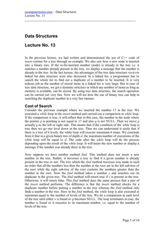
  • 7. Fig 13.3: Preorder: 14 4 3 9 7 5 15 18 16 17 20 14 154 9 7 183 5 16 20 17 ecomputernotes.com – Data Structures Lecture No. 13 ___________________________________________________________________ As all of these above routines are function so we will call them as: cout << "inorder: "; preorder( root); cout << "inorder: "; inorder( root ); cout << "postorder: "; postorder( root ); Here the root represents the root node of the tree. The size of the tree does not matter as the complete tree will be printed in preorder, inorder and postorder. Let’s discuss an example to see the working of these routines. Example Let’s have a look on the following tree. This is the same tree we have been using previously. Here we want to traverse the tree. In the bottom of the figure, the numbers are printed with the help of preorder method. These numbers are as 14 4 3 9 7 5 15 18 16 17 20. Now take these numbers and traverse the tree. In the preorder method, we print the root, followed by traversing of the left subtree and the right subtree respectively. As the value of the root node is 14, so it will be printed first of all. After printing the value of the root node, we call the preorder for the left node which is 4. Forget the node 14 as the root is 4 now. So the value 4 is printed and we call the preorder again with the left sub tree i.e. the node with value 3. Now the root is the node with value 3. We will print its value before going to its left. The left side of node with value 3 is NULL. Preorder will be called if condition Page 7 of 10
  • 8. Fig 13.4: Inorder: 3 4 5 7 9 14 15 16 17 18 20 14 154 9 7 183 5 16 20 17 ecomputernotes.com – Data Structures Lecture No. 13 ___________________________________________________________________ is false. In this case, no action will be taken. Now the preorder of the left subtree is finished. As the right subtree of this node is also NULL, so there is no need of any action. Now the left subtree of the node with value 4 is complete. The method preorder will be called for the right subtree of the node with value 4. So we call the preorder with the right node of the node with value 4. Here, the root is the node with value 9 that is printed. We will call its left subtree where the node value is 7. It will be followed by its left subtree i.e. node 5 which will be printed. In the preorder method, we take the root i.e. 14 in this case. Its value is printed, followed by its left subtree and so on. This activity takes us to the extreme left node. Then we back track and print the right subtrees. Let’s try to understand the inorder method from the following statement. When we call the inorder function, the numbers will be printed as 3 4 5 7 9 14 15 16 17 18 20. You might have noted that these numbers are in sorted order. When we build the tree, there was no need of sorting the numbers. But here we have the sorted numbers in the inorder method. While inserting a new node, we compare it with the existing ones and place the new node on the left or right side. So during the process of running the inorder on the binary tree, a programmer gets the numbers sorted. Therefore we have a sorting mechanism. If we are given some number, it will not be difficult to get them sorted. This is a new sorting algorithm for you. It is very simple. Just make BST with these numbers and run the inorder traversal. The numbers obtained from the inorder traversal are sorted. In the inorder method, we do not print the value of node first. We go to traverse its left subtree. When we come back from the left subtree and print the value of this node. Afterwards, we go to the right subtree. Now consider the above tree of figure 13.4. If we start from number 14, it will not be printed. Then we will go to the left subtree. The left subtree is itself a tree. The number 4 is its root. Now being at the node 4, we again look if there is any left subtree of this node. If it has a left subtree, we will not Page 8 of 10
  • 9. ecomputernotes.com – Data Structures Lecture No. 13 ___________________________________________________________________ print 4 and call the inorder method on its left subtree. As there is a left subtree of 4 that consists a single node i.e. 3, we go to that node. Now we call the inorder of node 3 to see if there is a subtree of it. As there is no left subtree of 3, the if statement that checks if the node is not NULL will become false. Here the recursive calls will not be executed. We will come back from the call and print the number 3. Thus the first number that is printed in the inorder traversal is 3. After printing 3, we go to its right subtree that is also NULL. So we come back to node 3. Now as we have traversed the left and right subtrees of 3 which itself is a left subtree of 4, thus we have traversed the left subtree of 4. Now we print the value 4 and go to the right subtree of 4. We come at node 9. Before printing 9 we go to its left subtree that leads us to node 7. In this subtree with root 7, we will not print 7. Now we will go to its left subtree which is node 5. We look for the left subtree of 5 which is NULL. Now we print the value 5. Thus, we have so far printed the numbers 3, 4 and 5. Now we come back to 7. After traversing its left subtree, we print the number 7. The right subtree of 7 is NULL. Thus finally, we have traversed the whole tree whose root is 7. It is a left subtree of 9. Now, we will come back to 9 and print it (as its left subtree has been traversed). The right subtree of 9 is NULL. So there is no need to traverse it. Thus the whole tree having 9 as its root has been traversed. So we come back to the root 4, the right subtree of which is the tree with root 9. Resultantly, the left and right subtree of 4 have been traversed now. Thus we have printed the numbers 3, 4, 5, 7 and 9. Now from here (i.e. node 4) we go to the node 14 whose left subtree has been traversed. Now we print 14 and go to its right subtree. The right subtree of 14 has 15 as the root. From here, we repeat the same process earlier carried out in case of the left subtree of 14. As a result of this process, the numbers 15, 16, 17, 18 and 20 are printed. Thus we get the numbers stored in the tree in a sorted order. And we get the numbers printed as 3, 4, 5, 7, 9, 14, 15, 16, 17, 18, 20. This sorted order is only in the inorder traversal. When we apply the post order traversal on the same tree, the numbers we get are not in sorted order. The numbers got through postorder traversal are in the following order: 3 5 7 9 4 17 16 20 18 15 14 We see that these are not in a sorted order. We know that every function has a signature. There is return type, function name and its parameter list in the signature of a function. Then there comes the body of the function. In the body of a function, there may be local variables and calls to some other functions. Now if a statement in the body of a function is calling the same function in which it exists, it will be termed as a recursive call. For example if a statement in function A is calling the function A, it is a recursive call and the process is called recursion. Now let’s see how recursion is carried out. We know that the function calls are implemented through stacks at run time. Let’s see what happens when there is a recursive call. In a recursive call that means calling a function itself makes no difference as far as the call stack is concerned. It is the same as a function F calls a function G, only with the difference that now function F is calling to function F instead of G. The following figure shows the stack layout when function F calls function F recursively. Page 9 of 10
  • 10. ecomputernotes.com – Data Structures Lecture No. 13 ___________________________________________________________________ Fig 13.5 When F is called first time, the parameters, local variables and its return address are put in a stack, as some function has called it. Now when F calls F, the stack will increase the parameters, local variables and return address of F comes in the stack again. It is the second call to F. After coming back from this second call, we go to the state of first call of F. The stack becomes as it was at first call. In the next lecture, we will see the functionality of recursive calls by an example. Exercise Please find out the preorder, inorder and postorder traversal of the tree given below: Page 10 of 10 Parameters(F) Local variables(F) Return address(F) Parameters(F) Parameters(F) Return address(F) Parameters(F) Local variables(F) Return address(F) Parameters(F) Local variables(F) Return address(F) During execution of F After callAt point of call sp sp sp Local variables(F) Fig 13.6 40 5014 19 17 8010 15 60 200 70 12 11 16 45 46 55 42 44