Engineering Mathematics 1

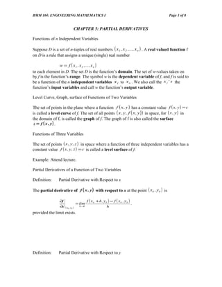
1. BMM 104: ENGINEERING MATHEMATICS I Page 1 of 8
CHAPTER 5: PARTIAL DERIVATIVES
Functions of n Independent Variables
Suppose D is a set of n-tuples of real numbers ( x1 , x 2 ,..., x n ) . A real valued function f
on D is a rule that assigns a unique (single) real number
w = f ( x1 , x 2 ,..., x n )
to each element in D. The set D is the function’s domain. The set of w-values taken on
by f is the function’s range. The symbol w is the dependent variable of f, and f is said to
be a function of the n independent variables x1 to x n . We also call the x j ' s the
function’s input variables and call w the function’s output variable.
Level Curve, Graph, surface of Functions of Two Variables
The set of points in the plane where a function f ( x , y ) has a constant value f ( x , y ) = c
is called a level curve of f. The set of all points ( x , y , f ( x , y ) ) in space, for ( x , y ) in
the domain of f, is called the graph of f. The graph of f is also called the surface
z = f ( x , y) .
Functions of Three Variables
The set of points ( x , y , z ) in space where a function of three independent variables has a
constant value f ( x , y , z ) = c is called a level surface of f.
Example: Attend lecture.
Partial Derivatives of a Function of Two Variables
Definition: Partial Derivative with Respect to x
The partial derivative of f ( x , y ) with respect to x at the point ( x0 , y 0 ) is
∂f f ( x0 + h , y 0 ) − f ( x0 , y 0 )
= lim ,
∂x ( x0 , y0 )
h→0 h
provided the limit exists.
Definition: Partial Derivative with Respect to y

2. BMM 104: ENGINEERING MATHEMATICS I Page 2 of 8
The partial derivative of f ( x , y ) with respect to y at the point ( x0 , y0 ) is
∂f d f ( x0 , y 0 + h ) − f ( x0 , y 0 )
= f ( x0 , y ) = lim ,
∂y ( x0 , y0 ) dy y = y0 h→0 h
provided the limit exists.
Example:
∂f ∂f
1. Find the values of and ∂ at the point ( 4 ,− ) if
5
∂x y
f ( x , y ) = x 2 + 3 xy + y − 1 .
∂ f
2. Find if f ( x , y ) = y sin xy .
∂ x
2y
3. Find f x and f y if f ( x , y ) = y + cos x .
Functions of More Than Two Variables
Example:
∂f ∂f ∂f
1. Let f ( x , y , z ) = xy 2 z 3 . Find , ∂ and at (1,− ,− ) .
2 1
∂x y ∂z
y
2. Let g ( x , y , z ) = x 2 e z . Find g x , g y and g z .
Second-Order Partial Derivatives
When we differentiate a function f ( x , y ) twice, we produce its second-order
derivatives.
These derivatives are usually denoted by
∂2 f f xx
“ d squared fdx squared “ or “f sub xx “
∂x 2
∂2 f
“ d squared fdy squared “ or f yy “f sub yy “
∂ 2
y
∂2 f f xx
“ d squared fdx squared “ or “f sub xx “
∂x 2
∂ f
2
“ d squared fdxdy squared “ or f yx “f sub yx “
∂∂
x y

3. BMM 104: ENGINEERING MATHEMATICS I Page 3 of 8
∂ f
2
“ d squared fdydx squared “ or f xy “f sub xy “
∂∂
y x
The defining equations are
∂2 f ∂  ∂f  ∂2 f ∂ ∂ 
f
=  , = 
∂ 
∂x 2
∂x  ∂x  ∂∂
x y ∂  y
x 
and so on. Notice the order in which the derivatives are taken:
∂ f
2
Differentiate first with respect to y, then with respect to x.
∂∂
x y
f yx = ( f y ) x Means the same thing.
Example:
∂2 f ∂ f
2
∂ f ∂ f
2 2
1. Let f ( x , y ) = x 3 y 2 − x 4 y 6 . Find , , and .
∂x 2 ∂ ∂ ∂
y x y2 ∂∂x y
∂2 f ∂ f
2
∂2 f ∂ f
2
2. If f ( x , y ) = x cos y + ye x , find , , and .
∂x 2 ∂ ∂ ∂
y x y2 ∂∂x y
The Chain Rule
Chain Rule for Functions of Two Independent Variables
If w = f ( x , y ) has continuous partial derivatives f x and f y and if x = x( t ) , y = y ( t )
are
differentiable functions of t, then the compose w = f ( x( t ) , y ( t ) ) is a differentiable
function of t and
df
= f x ( x ( t ) , y ( t ) ) • x ' ( t ) + f y ( x( t ) , y ( t ) ) • y ' ( t ) ,
dt
or
dw ∂f dx ∂f dy
= + .
dt ∂x dt ∂y dt
Example:
Use the chain rule to find the derivative of w = xy , with respect to t along the path

4. BMM 104: ENGINEERING MATHEMATICS I Page 4 of 8
π
x = cos t , y = sin t . What is the derivative’s value at t = ?
2
Chain Rule for Functions of Three Independent Variables
If w = f ( x , y , z ) is differentiable and x, y and z are differentiable functions of t, then w
is
a differentiable function of t and
dw ∂f dx ∂f dy ∂f dz
= + + .
dt ∂x dt ∂y dt ∂z dt
Example:
dw
Find if w = xy + z , x = cos t , y = sin t , z =t.
dt
Chain Rule for Two Independent Variables and Three Intermediate Variables
Suppose that w = f ( x , y , z ) , x = g ( r , s ) , y = h( r , s ) , and z = k ( r , s ) . If all four
functions
are differentiable, then w has partial derivatives with respect to r and s, given by the
formulas
∂w ∂ ∂
w x ∂ ∂w y ∂ ∂
w z
= + +
∂r ∂ ∂
x r ∂ ∂
y r ∂ ∂
z r
∂w ∂ ∂
w x ∂ ∂w y ∂ ∂
w z
= + +
∂s ∂ ∂
x s ∂ ∂
y s ∂ ∂
z s
Example:
∂w ∂w
Express and in terms of r and s is
∂r ∂s
r
w = x +2y + z2, x = , y = r 2 + ln s , z = 2 r .
s
If w = f ( x , y ) , x = g ( r , s ) , and y = h( r , s ) , then
∂w ∂ ∂
w x ∂ ∂
w y ∂w ∂ ∂
w x ∂ ∂
w y
= + and = +
∂r ∂ ∂
x r ∂ ∂
y r ∂s ∂ ∂
x s ∂ ∂
y s
Example:
∂w ∂w
Express and in terms of r and s if
∂r ∂s

5. BMM 104: ENGINEERING MATHEMATICS I Page 5 of 8
w = x2 + y2 , x= r− s, y =r+s.
If w = f ( x ) and x = g ( r , s ) , then
∂w dw ∂x ∂w dw ∂x
= and = .
∂r dx ∂r ∂s dx ∂s
PROBLEM SET: CHAPTER 5
1. Sketch and name the surfaces
(a) f ( x, y , z ) = x 2 + y 2 + z 2 (e) f ( x, y, z ) = x 2 + y 2
(b) f ( x , y , z ) = ln( x 2 + y 2 + z 2 ) (f) f ( x, y, z ) = y 2 + z 2
(c) f ( x, y , z ) = x + z (g) f ( x, y, z ) = z − x 2 − y 2
x2 y2 z2
(d) f ( x, y, z ) = z (h) f ( x, y , z ) = + +
25 16 9
∂f ∂f
2. Find and ∂ .
∂x y
(a) f ( x , y ) = 5 xy − 7 x 2 − y 2 + 3 x − 6 y + 2
y
(b) f ( x , y ) = tan −1  
x
(c) f ( x, y) = e ( x + y +1)
(d) f ( x , y ) = e −x sin( x + y )
(e) f ( x , y ) = ln( x + y )
(f) f ( x , y ) = sin 2 ( x − 3 y )
3. Find f x , f y and f z .
(a) f ( x , y , z ) = sin −1 ( xyz )
f ( x , y , z ) = e −( x )
2
+ y 2 +z 2
(b)
(c) f ( x , y , z ) = e −xyz
(d) f ( x , y , z ) = tanh( x + 2 y + 3 z )
4. Find all the second-order partial derivatives of the following functions.
(a) f ( x , y ) = x + y + xy
(b) f ( x , y ) = sin xy
(c) f ( x , y ) = x 2 y + cos y + y sin x

6. BMM 104: ENGINEERING MATHEMATICS I Page 6 of 8
(d) f ( x , y ) = xe y + y + 1
5. Verify that w xy = w yx .
(a) w = ln( 2 x + 3 y ) (c) w = xy 2 + x 2 y 3 + x 3 y 4
(b) w = e x + x ln y + y ln x (d) w = x sin y + y sin x + xy
dw
6. In the following questions, (a) express as a function of t, both by using
dt
the Chain Rule and by expressing w in terms of t and differentiating directly with
dw
respect to t. The (b) evaluate at the given value of t.
dt
(i) w = x2 + y2 , x = cos t , y = sin t ; t=π .
x y 1
(ii) w= + , x = cos 2 t , y = sin 2 t , z= t =3.
z z t
∂z ∂z
7. In the following questions, (a) express and as a functions of u and v
∂u ∂v
both by using the Chain Rule and by expressing z directly in terms of u and v
∂z ∂z
before differentiating. Then (b) evaluate and at the given point (u , v ) .
∂u ∂v
(i) z = 4 e x ln y , x = ln( u cos v ) , y = u sin v ; ( u ,v ) =  2 , π 
 
 4
(ii)
x
z = tan −1   ,
y x = u cos v , y = u sin v ; ( u ,v ) = 1.3 , π 
 
   6
ANSWERS FOR PROBLEM SET: CHAPTER 5
∂f ∂f
2. (a) = 5 y − 14 x + 3 , = 5 x − 2 y −6
∂x ∂y
∂f y ∂f x
(b) =− 2 , = 2
∂x x + y 2 ∂y x + y2
∂f ∂f
(c) = e ( x +y +1) , = e ( x +y +1 )
∂x ∂y
∂f ∂f
(d) = −e −x sin( x + y ) + e −x cos ( x + y ) , = e −x cos ( x + y )
∂x ∂y
∂f 1 ∂f 1
(e) = , =
∂x x + y ∂y x+y
∂f ∂f
(f) = 2 sin( x − 3 y ) cos( x − 3 y ) , = −6 sin( x − 3 y ) cos( x − 3 y )
∂x ∂x

7. BMM 104: ENGINEERING MATHEMATICS I Page 7 of 8
yz xz xy
3. (a) fx = , fy = , fz =
1−x y z2 2 2
1−x y z
2 2 2
1 − x2 y2 z2
f x = −2 xe −( x ) , f = −2 ye −( x f z = −2 ze − ( x + y + z )
(b)
2
+ y 2 +z 2 2
+ y 2 +z 2 ) , 2 2 2
y
(c) f x = −yze −xyz , f y = −xze −xyz , f z = −xye − xyz
(d) f x = sec h 2 ( x + 2 y + 3 z ) , f y = 2 sec h 2 ( x + 2 y + 3 z ) ,
f z = 3 sec h 2 ( x + 2 y + 3 z )
∂f ∂f ∂2 f
=1 + x , ∂ f = 0,
2
∂2 f ∂2 f
4. (a) = 1 + y, = 0, = =1
∂x ∂y ∂x 2 ∂y 2 ∂∂
y x ∂∂
x y
∂f ∂f ∂2 f
= x cos xy , ∂ f = − y 2 sin xy ,
2
(b) = y cos xy , = −x 2 sin xy ,
∂x ∂y ∂x 2 ∂y 2
∂2 f ∂2 f
= = cos xy − xy sin xy
∂y∂x ∂x∂y
∂f ∂f
= x 2 − sin y + sin x , ∂ f = 2 y − y sin x ,
2
(c) = 2 xy + y cos x ,
∂x ∂y ∂x 2
∂ f
2
∂2 f ∂2 f
= −cos y , = = 2 x + cos x
∂y 2
∂y∂x ∂x∂y
∂f ∂f ∂2 f
= xe y + 1 , ∂ f = 0 ,
2
∂2 f ∂2 f
(d) =ey = xe y , = =e y
∂x ∂y ∂x 2 ∂y 2
∂∂
y x ∂∂
x y
∂w 2 ∂w 3 ∂2 w −6
5. (a) = , = , = , and
∂x 2 x + 3 y ∂y 2 x + 3 y ∂y∂x (2x + 3 y) 2
∂2 w −6
=
∂x∂y ( 2 x + 3 y ) 2
∂w y ∂w x ∂2 w 1 1
(b) = e x + ln y + , = + ln x , = + , and
∂x x ∂y y ∂∂
y x y x
∂2w 1 1
= +
∂x∂y y x
∂w ∂w
(c) = y 2 + 2 xy 3 + 3 x 2 y 4 , = 2 xy + 3 x 2 y 2 + 4 x 3 y 3 ,
∂x ∂y
∂2 w ∂2 w
= 2 y + 6 xy 2 + 12 x 2 y 3 , and = 2 y + 6 xy 2 + 12 x 2 y 3
∂y∂x ∂x∂y

8. BMM 104: ENGINEERING MATHEMATICS I Page 8 of 8
∂w ∂w
(d) = sin y + y cos x + y , = x cos y + sin x + x ,
∂x ∂y
∂2 w ∂2 w
= cos y + cos x + 1, and = cos y + cos x + 1
∂y∂x ∂x∂y
dw
6. (i) (a) =0 (b) 0
dt
dw
(ii) (a) =1 (b) 1
dt
∂z
7. (i) (a) = ( 4 cos v ) ln( u sin v ) + 4 cos v
∂u
∂z 4u cos 2 v
= ( − 4u sin v ) ln( u sin v ) +
∂v sin v
∂z
(b) = 2 ( ln 2 + 2 )
∂u
∂z
= −2 2 ln 2 + 4 2
∂v
∂z
(ii) (a) =0
∂u
∂z
= −1
∂v
∂z
(b) =0
∂u
∂z
= −1
∂v

9. BMM 104: ENGINEERING MATHEMATICS I Page 8 of 8
∂w ∂w
(d) = sin y + y cos x + y , = x cos y + sin x + x ,
∂x ∂y
∂2 w ∂2 w
= cos y + cos x + 1, and = cos y + cos x + 1
∂y∂x ∂x∂y
dw
6. (i) (a) =0 (b) 0
dt
dw
(ii) (a) =1 (b) 1
dt
∂z
7. (i) (a) = ( 4 cos v ) ln( u sin v ) + 4 cos v
∂u
∂z 4u cos 2 v
= ( − 4u sin v ) ln( u sin v ) +
∂v sin v
∂z
(b) = 2 ( ln 2 + 2 )
∂u
∂z
= −2 2 ln 2 + 4 2
∂v
∂z
(ii) (a) =0
∂u
∂z
= −1
∂v
∂z
(b) =0
∂u
∂z
= −1
∂v

10. BMM 104: ENGINEERING MATHEMATICS I Page 8 of 8
∂w ∂w
(d) = sin y + y cos x + y , = x cos y + sin x + x ,
∂x ∂y
∂2 w ∂2 w
= cos y + cos x + 1, and = cos y + cos x + 1
∂y∂x ∂x∂y
dw
6. (i) (a) =0 (b) 0
dt
dw
(ii) (a) =1 (b) 1
dt
∂z
7. (i) (a) = ( 4 cos v ) ln( u sin v ) + 4 cos v
∂u
∂z 4u cos 2 v
= ( − 4u sin v ) ln( u sin v ) +
∂v sin v
∂z
(b) = 2 ( ln 2 + 2 )
∂u
∂z
= −2 2 ln 2 + 4 2
∂v
∂z
(ii) (a) =0
∂u
∂z
= −1
∂v
∂z
(b) =0
∂u
∂z
= −1
∂v

11. BMM 104: ENGINEERING MATHEMATICS I Page 8 of 8
∂w ∂w
(d) = sin y + y cos x + y , = x cos y + sin x + x ,
∂x ∂y
∂2 w ∂2 w
= cos y + cos x + 1, and = cos y + cos x + 1
∂y∂x ∂x∂y
dw
6. (i) (a) =0 (b) 0
dt
dw
(ii) (a) =1 (b) 1
dt
∂z
7. (i) (a) = ( 4 cos v ) ln( u sin v ) + 4 cos v
∂u
∂z 4u cos 2 v
= ( − 4u sin v ) ln( u sin v ) +
∂v sin v
∂z
(b) = 2 ( ln 2 + 2 )
∂u
∂z
= −2 2 ln 2 + 4 2
∂v
∂z
(ii) (a) =0
∂u
∂z
= −1
∂v
∂z
(b) =0
∂u
∂z
= −1
∂v