We analyse the temporal variations which can be observed within time series of variogram parameters (nugget, sill and range) of daily air quality data (PM10) over a ten years time frame.

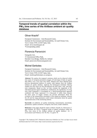
1. Int. J. Environment and Pollution, Vol. 58, Nos. 1/2, 2015 63
Copyright © The Authors(s) 2015. Published by Inderscience Publishers Ltd. This is an Open Access Article
distributed under the CC BY license. (http://creativecommons.org/licenses/by/4.0/)
Temporal trends of spatial correlation within the
PM10 time series of the AirBase ambient air quality
database
Oliver Kracht*
European Commission – Joint Research Centre,
Institute for Environment and Sustainability, Air and Climate Unit,
Via E. Fermi 2749, I-21027 Ispra, Italy
Email: oliver.kracht@gmx.de
*Corresponding author
Florencia Parravicini
Garageeks Ltd.,
31 Greenmount Office Park,
Harolds Cross Bridge, Dublin 6w, Ireland
Email: parravicini.florencia@gmail.com
Michel Gerboles
European Commission – Joint Research Centre,
Institute for Environment and Sustainability, Air and Climate Unit,
Via E. Fermi 2749, I-21027 Ispra, Italy
Email: michel.gerboles@jrc.ec.europa.eu
Abstract: We analyse the temporal variations which can be observed within
time series of variogram parameters (nugget, sill and range) of daily air quality
data (PM10) over a ten years time frame. Datasets have been obtained from
previous geostatistical analysis of country wide datasets from the AirBase
ambient air quality database. Applying the Kolmogorov-Zurbenko filtering
method, the time series are first decomposed into their short-, mid-, and long-
term components. Based on this, we then evaluate the magnitude of the
individual spectral signal contributions. Furthermore, the significance of a long
term trend component is investigated by a block-bootstrap-based approach
combined with linear regression. It is discussed if within these datasets
the times series of nugget variance can provide information about the
evolution of the measurement uncertainty of the related air pollutant, whereas
the sill and the range parameters could contain information about the spatial
representativeness of the monitoring stations.
Keywords: air pollution; air quality monitoring; measurements; uncertainty;
geostatistics; spatial correlation; variogram; time series; model validation.
Reference to this paper should be made as follows: Kracht, O., Parravicini, F.
and Gerboles, M. (2015) ‘Temporal trends of spatial correlation within the
PM10 time series of the AirBase ambient air quality database’, Int. J.
Environment and Pollution, Vol. 58, Nos. 1/2, pp.63–78.

2. 64 O. Kracht et al.
Biographical notes: Oliver Kracht has been a Postdoctoral Researcher at the
European Commission Joint Research Centre in Ispra (Italy) since 2012, where
he has been working on geostatistical methods for the evaluation of ambient
air quality data. He graduated from the Department of Geosciences at the
University of Bochum (Germany). Following an employment at the University
of Lausanne (Switzerland), he moved to the Swiss Federal Institute of Aquatic
Science and Technology. In 2007, he obtained his PhD in Environmental
Engineering from the ETH Zurich. He worked as a PostDoc at the University of
Bern (Switzerland), and as a Marie Curie Fellow at the Geological Survey of
Norway.
Florencia Parravicini holds a BSc in Life Sciences from the University of Pau
and Pays de l’Adour, France, and an MSc in Environmental Sciences from the
University of Insubria, Italy. She has worked at the European Commission
Joint Research Centre in Ispra (Italy) during years 2011 and 2012 and
contributed to the scientific research project ‘Geostatistics in Air Quality
Assessment’. She is currently developing an electronic prototype for air quality
monitoring by using simple, low-cost and mobile sensors connected to an
Arduino open-source hardware device.
Michel Gerboles graduated in Analytical Chemistry from the University of
Bordeaux (FR). In 1990, he joined the Joint Research Centre of the European
Commission, as quality officer of the European Reference Laboratory for Air
Pollution. His activities range from the improved calibration of primary
reference methods for air quality monitoring to the organisation of proficiency
testing and intercomparison exercises in support to the European policy on air
quality. His current research interests include the validation of novel
inexpensive gas sensor technologies, and the development of automatic
methods for the extraction of quality indicators from large ambient air
monitoring datasets.
This paper is a revised and expanded version of a paper entitled ‘Trends of
daily variogram parameters derived by geostatistical analysis of PM10 time
series from the AirBase ambient air quality database’ presented at the 16th
International Conference on Harmonisation within Atmospheric Dispersion
Modelling for Regulatory Purposes, Varna, Bulgaria, 8–11 September 2014.
1 Introduction
A common step in the evaluation of model performance and in model validation is to
compare the modelled results to observations obtained from air quality monitoring. In
this context, statistical indicators which aim to determine whether model results have
reached a sufficient level of agreement with the observations, require an estimate or an
assumption to be made for both the measurement uncertainties and the spatial
representativeness of the air quality parameters being used. Quantitative values for the
measurement uncertainty are usually derived from experimental work specifically
addressing the individual measurement techniques. Quantification of spatial
representativeness in conventional practice is frequently based on the evaluation of
specific site characteristics and assumptions being made about similarities of those
characteristics within the surrounding domains. However, in order to facilitate the
thorough exploitation of comprehensive observation datasets, the use of geostatistical

3. Temporal trends of spatial correlation within the PM10 time series 65
techniques can serve as an interesting alternative which can immediately be applied to the
monitoring data without need to refer to secondary information. The underlying idea is
that within such datasets the nugget variance can provide information about the
measurement uncertainty and the micro-scale variability of the related air quality
measurements, whereas the sill and the range parameter contain information about their
spatial representativeness [for a more detailed introduction to this conceptualisation
please refer to Gerboles and Reuter (2010)]. However, this information is assumed to be
obfuscated by several atmospheric processes which are superimposing the signal of
interest on a range of different time scales.
2 Geostatistical techniques
Geostatistics is a branch of applied statistics that quantifies the spatial dependence and
the spatial structure of a measured property. It is based on the regionalised variable
theory by which spatial correlation of measured properties can be treated (Matheron,
1963). Commonly, geostatistical analysis expresses the spatial correlation structure of the
observations of an environmental variable x (e.g., a pollutant concentration) in terms of
the variogram (sometimes also called the semivariogram). For this purpose the
experimental semivariance γ(l) is calculated to
( ) ( )[ ]
1
2
1
1 1
( )
2 ( )
n
i l i
i
γ l z x z x
n l
−
+
=
= −∑ (1)
where n(l) is the number of sample pairs at each lag distance l, and z(xi) and z(xi+l) are the
values of x at the locations i and i + l. It is usual to fit the experimental semivariance
values with a simple continuous model function in which the semi-variance γ is described
as a function of lag distance l (the theoretical variogram). In this context the Gaussian,
the exponential or the spherical variogram models are the most commonly used. The
spherical model [equation (2)] is often considered the best choice when spatial
autocorrelation decreases to a point after which it becomes zero.
( )3
0 1
0 1
( ) 1.5 0.5 if 0
( ) if
l l
a aγ l C C l a
γ l C C l a
⎡ ⎤= + − ≤ ≤⎣ ⎦
= + >
(2)
The parameters of the spherical model consist of the nugget C0, the partial sill C1, and the
range a. The nugget variance C0 represents the variability of the observations at small
distances (tending towards 0). The empirical nugget variance is unknown since it is the
value of the theoretical variogram at the origin. The nugget parameter C0 is thus
estimated by extrapolating the variogram towards l = 0. From this point, the semivariance
increases until the full sill variance C0 + C1 is reached at a lag distance called the range
(a). The range provides the distance beyond which semivariances remain constant. Up to
this distance, observations of the regionalised variable in the sampling locations are
correlated, afterwards they must be considered to be spatially independent. Note
specifically that the term partial sill (shorthand pSill) is used to denote C1, whereas the
term sill denotes C0 + C1.

4. 66 O. Kracht et al.
3 Material and methods
In this study, we analysed the temporal variations observed within time series of
variogram parameters obtained from different country wide datasets of daily average
PM10 data from the AirBase v.4 ambient air quality database. For the scope of this
exercise, it was decided to apply the evaluation to the sole stations of background type,
but for all area types (urban, suburban and rural). The assessment extends over a ten
years time frame (1997 to 2007) and considers data from six different countries (FR, DE,
GB, AT, IT and NL). The original material comprising comprehensive variogram
parameter sets with time series of nugget (C0), partial sill (C1), and range (a) had already
been established from variogram model fits within earlier projects (Gerboles et al., 2016).
In this primary work a spherical variogram model had been used. More details about
these previously reported analyses and about the underlying geostatistical computations
can be obtained from Gerboles and Reuter (2010) and from Kracht et al. (2014). An
overview about the number of variogram fits available within the ten years time frame is
given in Table 1.
Table 1 Overview of available variography sets (individual variogram models fitted to PM10
daily values), and summary of median values obtained for the nugget, partial sill and
range parameter
Country
Available variogram fits Summary of median values
First
available
[year]
Last
available
[year]
Available fits
[count]
Accepted fits
[count]
Nugget (2s)
[µg/m3
]
pSill (2s)
[µg/m3
]
Range
[deg]
FR 2001 2007 2,051 1,221 6.45 9.17 0.50
DE 1998 2007 3,232 1,555 6.99 9.25 0.82
GB 1997 2007 3,932 2,415 6.13 7.01 0.34
AT 2001 2007 2,280 1,189 8.29 11.31 0.66
IT 2003 2007 1,737 890 12.67 19.85 0.85
NL 2003 2007 1,258 1,235 7.97 8.29 -
Notes: Note that nugget and partial sill values have been converted from spatial variances
to standard deviations times two (2s) and are thus presented in units of [µg/m3
].
Constraints applied for accepting a valid variogram model fit have been:
(I) 1 < Nugget < 150 (µg/m3
)2
(II) 0 < pSill < 104
(µg/m3
)2
(III) 0.01 < Range < 2 deg
(IV) 0.04 < pSill/Nugget < 5·103
All simulation codes used in this study were developed in the R environment
(R Development Core Team, 2014). In order to extend the necessary capacities, we
included functionalities from the packages ‘kza’ (Close and Zurbenko, 2013), ‘boot’
(Canty and Ripley, 2013; Davison and Hinkley, 1997), and ‘Kendall’ (McLeod, 2011).
In a first step, the time series of variography parameters were screened for internal
consistency by applying a set of constraints (I, II, III, IV, see note in Table 1) for
accepting a valid variogram model fit (Table 1).
In a second preparatory step, the nugget and partial sill values of the accepted model
fits were converted from spatial variances to spatial standard deviations times two

5. Temporal trends of spatial correlation within the PM10 time series 67
[equation (3)]. This transformation was preferred for the convenience of the later
discussion (e.g. a comparison of nugget values to the uncertainty of measurements
derived from independent laboratory studies or field exploration studies). Note that
nugget and partial sill are thus presented in units of µg/m3
and that the shorthand ‘2s’ is
used to indicate that parameters have been transformed in this manner. Range values
remain untransformed and are expressed in units of spherical degrees.
0
1
(2 ) 2
(2 ) 2
Nugget s C
pSill s C
=
=
(3)
Using the Kolmogorov-Zurbenko (KZ) filtering method (Rao et al., 1997; Eskridge et al.,
1997) we then aimed to separate the original time series X(t) into its different components
[equation (4)].
( ) ( ) ( ) ( )X t e t S t W t= + + (4)
In this conceptualisation, the short-term component W(t) is attributable to variations of
weather and to short-term fluctuations in precursor emissions. The mid-term (seasonal)
component S(t) can be interpreted as a result of changes in the solar angle (induced
variations of emissions and temperature dependencies). The long-term signal e(t) can be
interpreted to result from long-term changes in overall emissions, pollutant transport,
climate, economics, and environmental policies (Wise and Comrie, 2005). e(t) is as
well supposed to be influenced by evolutions in the operational principles of the
monitoring network. In addition, Baseline(t) is defined as the sum of the long-term and
seasonal component. For the decomposition of the raw data time series, a KZ filter with
k = 5 iterations of a moving average window of m = 15 days (KZ[15,5]) was used for
extracting the baseline. A KZ[365,3] filter was used to obtain the long-term signal e(t).
Note that KZ[15,5] has a low pass periodicity of 34 days, while KZ[365,3] has a low pass
periodicity of 632 days.
Finally, the significances of long term trend components of the nugget and the sill and
range effect were investigated from the slope of linear regression lines fitted to each set
of the unfiltered time series X(t). This required specific care to be taken because of the
serial autocorrelation inherent in these data, which became evident from systematic
patterns observed in S(t). A simple linear regression would have all observations within
an individual time series of variogram parameter values assumed to be independent. This
is likely to give reasonable estimates of the regression coefficients, but to overstate their
significance. To obtain more accurate confidence intervals, we chose to combine linear
regression with a block-bootstrap-based approach (Künsch, 1989). In this way, the slope
parameter was estimated by ordinary linear regression applied to bootstrap replicates
chosen randomly from the original time series. We used a variable block length following
a geometric distribution with a mean value of 30 days (CF-Interval 1) and 365 days
(CF-Interval 2), respectively. Confidence intervals on the 95% level were then estimated
by applying a coverage factor of 1.96 to the empirical standard deviation of the
bootstrapped slope estimates. After some initial tests, it was considered suitable to
perform 10,000 resamplings per time series to obtain good stability in the significance
level estimates.

6. 68 O. Kracht et al.
4 Results and discussion
Figures 1, 2 and 3 are illustrating the decomposition and trend analysis being applied to
the nugget, partial sill and range time series of background stations from six different
countries (FR, DE, GB, AT, IT and NL). In addition, an overview of the medians
calculated for the raw parameter values of nugget, partial sill and range is given in
Table 1. Note that for convenience of discussion nugget and partial sill values have been
converted from variances to standard deviations times two and are thus presented in units
of µg/m3
.
As a first observation from the aggregated absolute values of spatial variation
(Table 1), both the nugget and the partial sill are highest for Austria and Italy. This
general characteristic is indicating limitations in the spatial continuity of the data. It
appears obvious that this effect could be due to the stronger topographic roughness and
dissection of these two countries. However, other possible causes could be considered,
like the impact of different sub-networks which might work independently and
potentially according to non-synchronised procedures, or the impact of the variety of
monitoring equipments and/or calibration techniques being used.
In contrast to these observations made for the nugget and partial sill, considering the
aggregated values from the whole time series, a similarly generalisable observation
cannot be made for the range parameter. This is actually because for some of the
countries a clear interpretation of the range parameter is complicated by a superimposed
trend component, as will be discussed later.
A closer look at the time series (Figures 1, 2 and 3) reveals that several data series
are showing a pronounced cyclic behaviour in their seasonal component S(t), and a
non-stationarity (change of variance over time) in their short-term component W(t). These
effects clearly indicate the presence of temporal variations in the macroscale spatial
correlation structures (partial sill and range). Furthermore, for the examples of Austria,
Italy, Germany and France, a distinct phase relationship of the S(t) component consisting
in a winter increase of the sill effect is observed. It is likely that spatial variability
increases in winter time because of local emission caused by heating, sanding and
particulate matter re-suspension, as well as by limited air mixing increasing the
discontinuity of PM10 concentration levels. However, for Austria and Italy this phase
relationship is also observed in the nugget effect time series, which might indicate the
influence of increasing small scale variability in winter time, too. Notably, in contrary to
the abovementioned observations made for the nugget and partial sill, a clear phase
relationship cannot be identified in the S(t) component of the range time series.
Exploring in more detail the nugget effect time series is indeed of high practical
interest, as it can provide information about the evolution of the average measurement
uncertainty of the related air pollutant (in this context average measurement uncertainty
refers to a characterisation across a country dataset, as opposed to the individual
measurement uncertainty of a single station). From a conceptual point of view, the two
dominant causes for the nugget effect do consist of the uncertainty of the measurements
and of the microscale variability (i.e. variations at distances smaller than the sampling
distance). For the generalised case it is actually difficult to distinguish the proportions
contributed by these two components, by using information obtained from geostatistics
and time series analysis only. However, in order to account for these difficulties and to
minimise the influence of small scale variability the datasets used in this exercise have
already been preselected to comprise background type stations only.

7. Temporal trends of spatial correlation within the PM10 time series 69
Figure 1 Time series of estimated nugget parameter values from spherical variogram models
fitted to PM10 daily values of AirBase v.4 background stations (see online version
for colours)
Notes: Nugget values have been converted from spatial variances to spatial standard
deviations times two (2s) and are in units of [µg/m3
]. The KZ[15,5] filter has a low
pass periodicity of 34 days that gives the baseline air quality. KZ[365,3] has a low
pass periodicity of 632 days. W(t) can be used to characterise the short-term
component, S(t) for the seasonal component, and e(t) reflects the long-term signal
and trend. Baseline(t) is defined as the sum of the long-term and seasonal
component.

8. 70 O. Kracht et al.
Figure 2 Time series of estimated partial sill parameter values from spherical variogram models
fitted to PM10 daily values of AirBase v.4 background stations (see online version
for colours)
Notes: Partial sill values have been converted from spatial variances to spatial standard
deviations times two (2s) and are in units of [µg/m3
]. The KZ[15,5] filter has a
low pass periodicity of 34 days that gives the baseline air quality. KZ[365,3] has a
low pass periodicity of 632 days. W(t) can be used to characterise the short-term
component, S(t) for the seasonal component, and e(t) reflects the long-term signal
and trend. Baseline(t) is defined as the sum of the long-term and seasonal
component.

9. Temporal trends of spatial correlation within the PM10 time series 71
Figure 3 Time series of estimated range parameter values from spherical variogram models fitted
to PM10 daily values of AirBase v.4 background stations. Range values are presented in
units of geographical coordinates [deg] (see online version for colours)
Notes: Data for the Netherland have been omitted, because of convergence problems
observed with the variogram fitting algorithm applied to this country (singularities
due to a correlation between the sill and range estimates in this specific dataset).
The KZ[15,5] filter has a low pass periodicity of 34 days that gives the baseline
air quality. KZ[365,3] has a low pass periodicity of 632 days. W(t) can be used to
characterise the short-term component, S(t) for the seasonal component, and e(t)
reflects the long-term signal and trend. Baseline(t) is defined as the sum of the
long-term and seasonal component.

10. 72 O. Kracht et al.
Interpretations of seasonal effects on the spatial correlation lengths and on the small scale
variability of the actual PM10 concentrations have been discussed in the previous
paragraph. Nevertheless, the observed short term influences (non-stationarities) and
seasonal variations in the nugget time series are equally well compatible with the
assumption of related short term influences and seasonal fluctuations of the measurement
uncertainty. Indeed, as the composition and properties of particulate matter and ambient
parameters (like temperature and relative humidity) vary in time, they do as well
influence the uncertainty of the different PM10 mass measurements principles (Pernigotti
et al., 2013).
The magnitudes of the individual spectral signal contributions to the temporal
variation of the nugget, partial sill and range parameter time series can be compared from
the overall variance calculated for each of the filter-separated time series. Table 2
provides an overview of the observed temporal variances. In addition, Table 3
summarises normalised values, for which the total values of the four filter-separated
spectral components have been adjusted by division with the total variance of the
corresponding raw values. Example given for interpretation, the seasonal component S(t)
is strongly pronounced within the data series of Austria and Italy (absolute values in
Table 2). Also the short term component W(t) has its largest expression in the datasets of
these latter two countries. In analogy to the interpretation of the median parameters of the
total spatial variation (Table 1), we consider that this observation once more indicates a
lack of spatial continuity of PM10 most likely due to the stronger topographic roughness
and dissection as compared to the other countries. However, as discussed before with
regard to the evaluation in the time domain, an influence by the effects of different PM10
measurements principles cannot be finally ruled out.
Table 2 Overall temporal variance of the raw variogram parameter estimates and of the
filtered time series
Country Parameter
Raw values
[(µg/m3
)2
]
Baseline
[(µg/m3
)2
]
e(t)
[(µg/m3
)2
]
S(t)
[(µg/m3
)2
]
W(t)
[(µg/m3
)2
]
FR Nugget (2s) 2.51 1.48 0.14 0.46 1.16
DE Nugget (2s) 3.28 0.94 0.08 0.73 1.96
GB Nugget (2s) 2.87 0.43 0.03 0.34 2.16
AT Nugget (2s) 5.41 1.95 0.06 2.28 3.17
IT Nugget (2s) 6.50 2.09 0.01 2.34 4.28
NL Nugget (2s) 2.92 0.47 0.00 0.30 2.21
FR pSill (2s) 5.98 1.99 0.19 1.33 2.76
DE pSill (2s) 13.95 3.86 0.14 4.00 7.32
GB pSill (2s) 6.50 0.73 0.05 0.57 5.04
AT pSill (2s) 30.47 15.29 0.34 16.44 13.58
IT pSill (2s) 53.66 26.47 0.54 29.76 26.16
NL pSill (2s) 8.38 0.94 0.01 0.74 6.63
Notes: The time series have not been de-trended for these calculations. Note that because
nugget and partial sill values have been converted from spatial variances to
standard deviations times two (2s), the unit for the temporal variance of the time
series is (µg/m3
)2
.

11. Temporal trends of spatial correlation within the PM10 time series 73
Table 2 Overall temporal variance of the raw variogram parameter estimates and of the
filtered time series (continued)
Country Parameter
Raw values
[deg2
]
Baseline
[deg2
]
e(t)
[deg2
]
S(t)
[deg2
]
W(t)
[deg2
]
FR Range 0.58 0.33 0.16 0.21 0.47
DE Range 0.63 0.30 0.20 0.21 0.55
GB Range 0.53 0.19 0.06 0.16 0.48
AT Range 0.56 0.23 0.06 0.20 0.49
IT Range 0.57 0.22 0.04 0.20 0.51
NL Range - - - - -
Notes: The time series have not been de-trended for these calculations. Note that because
nugget and partial sill values have been converted from spatial variances to
standard deviations times two (2s), the unit for the temporal variance of the time
series is (µg/m3
)2
.
Table 3 Normalised temporal variance of the raw variogram parameter estimates and of the
filtered time series
Country Parameter
Raw values
[normalised]
Baseline
[normalised]
e(t)
[normalised]
S(t)
[normalised]
W(t)
[normalised]
FR Nugget (2s) 1 0.59 0.06 0.18 0.46
DE Nugget (2s) 1 0.29 0.02 0.22 0.60
GB Nugget (2s) 1 0.15 0.01 0.12 0.75
AT Nugget (2s) 1 0.36 0.01 0.42 0.59
IT Nugget (2s) 1 0.32 0.00 0.36 0.66
NL Nugget (2s) 1 0.16 0.00 0.10 0.75
FR pSill (2s) 1 0.33 0.03 0.22 0.46
DE pSill (2s) 1 0.28 0.01 0.29 0.52
GB pSill (2s) 1 0.11 0.01 0.09 0.78
AT pSill (2s) 1 0.50 0.01 0.54 0.45
IT pSill (2s) 1 0.49 0.01 0.55 0.49
NL pSill (2s) 1 0.11 0.00 0.09 0.79
FR Range 1 0.57 0.28 0.36 0.81
DE Range 1 0.48 0.32 0.33 0.87
GB Range 1 0.36 0.11 0.30 0.91
AT Range 1 0.41 0.11 0.36 0.88
IT Range 1 0.39 0.07 0.35 0.89
NL Range - - - - -
Notes: For this table, all temporal variances have been normalised by the temporal
variance of the raw values. Note that the time series have not been de-trended
for these calculations.
In contrast to these observations made for Austria and Italy, Great Britain and the
Netherlands are characterised by the lowest absolute seasonal variation S(t) of the nugget

12. 74 O. Kracht et al.
and the partial sill parameter (Table 2). On the other hand, because of this weakly
pronounced S(t) component, the relative importance of W(t) is most prominent for these
two countries (normalised values in Table 3). Finally, for the range parameter, results
from Tables 2 and 3 suggest that the magnitudes of signal contributions from the seasonal
and short term components (S(t) and W(t)) are more homogenously distributed across the
different countries. However, the range parameters of France and Germany reveal a
significant trend signal e(t), as will be discussed in more detail later.
Results of the trend analysis are presented in Table 4. A significant trend component
could only be found in the nugget time series of France (a negative slope of –0.73 ± 0.31
µg/m3
/year) and Great Britain (a slightly positive slope of 0.11 ± 0.09 µg/m3
/year), and in
the range time series of France (a positive slope of 0.13 ± 0.03 deg/year) and Germany
(a positive slope of 0.05 ± 0.03 deg/year). For all other series the slope of the linear trend
component was not significant in consideration of the bootstrapped confidence intervals.
As an important note, the expressiveness of the trend analyses was somewhat limited by
the relatively short extend of the valid variogram time series for some of the countries.
Table 4 Summary of the bootstrap-based trend analyses performed on the nugget, partial sill
and range parameter time series
Country Parameter
Trend slope
[µg/m3
/year]
95% Conf-Int-1
[µg/m3
/year]
95% Conf-Int-2
[µg/m3
/year]
Significant?
FR Nugget (2s) –0.73 ±0.24 ±0.31 Yes
DE Nugget (2s) –0.02 ±0.18 ±0.28 No
GB Nugget (2s) 0.11 ±0.07 ±0.09 Yes
AT Nugget (2s) –0.09 ±0.41 ±0.47 No
IT Nugget (2s) –0.09 ±0.51 ±0.56 No
NL Nugget (2s) –0.11 ±0.30 ±0.41 No
FR pSill (2s) –0.28 ±0.44 ±0.63 No
DE pSill (2s) 0.13 ±0.36 ±0.45 No
GB pSill (2s) –0.01 ±0.11 ±0.15 No
AT pSill (2s) 0.11 ±1.04 ±1.06 No
IT pSill (2s) 0.54 ±1.89 ±2.28 No
NL pSill (2s) 0.00 ±0.45 ±0.35 No
[deg/year] [deg/year] [deg/year]
FR Range 0.13 ±0.02 ±0.03 Yes
DE Range 0.05 ±0.02 ±0.03 Yes
GB Range –0.02 ±0.01 ±0.02 No
AT Range 0.02 ±0.03 ±0.04 No
IT Range –0.01 ±0.05 ±0.08 No
NL Range - - - -
Notes: The 95% confidence intervals Conf-Int-1 and Conf-Int-2 are corresponding to a
resampling with mean block lengths of 30 days and 365 days respectively.
A negative trend in the nugget time series can be interpreted by an improvement of the
measurement uncertainty of the monitoring stations over the years, but also by a

13. Temporal trends of spatial correlation within the PM10 time series 75
reduction in small scale variability (change in the nature or quantity of emissions,
transported pollution, or atmospheric reactions). Other reasons causing either negative or
positive trends might be the increase/decrease of the number of monitoring stations or a
change in the station classifications. A positive trend in the range time series indicates
that measurements of stations are becoming more homogeneous. This can be caused by
an increase of quality actions performed on the measuring stations over the years.
However, as for the nugget time series, a trend of the range values might also be the
result of a change in the nature or quantity of emissions, pollution transport, or
atmospheric reactions, as well as it could result from an increase/decrease of the number
of monitoring stations or from a change in the station classifications.
Figure 4 Time series of the number of stations available for the analysis
Note: Note that if less than 20 stations were available at a given time step (i.e. day), the
semi-variogram analysis was not performed.

14. 76 O. Kracht et al.
In a final analysis, we counterchecked to which extent the trend analysis could have been
affected by factors related to temporal fluctuations in data availability. Figure 4 provides
time series of the number of stations available for the geostatistical analysis per day. As a
general observation, the amount of monitoring stations available increases over time.
This has a direct influence on the feasibility of the variogram parameter estimation. In
fact the algorithm used in Gerboles and Reuter (2010) constrained the geostatistical
analysis to those days with a minimum number of 20 stations being available. Example
given, it is for this reason that the variogram analysis for the Netherlands dataset was not
feasible for time sections before ca summer 2003. On the other hand, nearly all
Netherland data fulfilling this constrained subsequently delivered a valid variogram
model fit, which can be explained by the prevailing spatial continuity of PM10 data for
this country.
Within a given network the number of monitoring stations is directly linked with the
distribution of distances between these stations. Against this background, the nugget
parameter C0 needs to be considered as being an extrapolated value. Consequently, the
accuracy of its estimation depends on the semi-variance at the smallest lag distance.
According to the evolution of network design and station density, the time series will
present different smallest lags at different times (in a first order approximation all
datasets share a decrease of lag distance over time). Therefore one cannot exclude a lack
of homogeneity of the extrapolated nugget variance according to the smallest lag
distance. However, even though these effects can influence the accuracy of the individual
estimates, they are not supposed to result in a systematic bias towards higher of lower
values.
5 Summary and conclusions
Temporal variations in the spatial autocorrelation structure of air quality data can reflect
changes in the performance and operational conditions of a monitoring network
(improvement or worsening of the measurement uncertainty, increase/decrease of the
number of monitoring stations, positioning of stations, and shifting in the station
classification). However, these phenomena are interfering with changes of the spatial
distribution of air pollutants due to transport, emissions and reactions.
In this exploratory study we investigated time series of variogram parameters by
applying the Kolmogorov-Zurbenko filtering method. Furthermore, the significance of
long term trend components was investigated by a block-bootstrap-based approach
combined with linear regression. A significant trend component was found in the nugget
time series of France (decrease) and Great Britain (slight increase), and in the range time
series of France and Germany (both increasing). Furthermore, a pronounced cyclic
behaviour of the seasonal time series component was detected. This seasonal effect is
associated with a phase relationship (winter increase) of the nugget and of the partial sill
series for several countries, which is particularly pronounced for Austria and Italy. Such
effects are likely attributable to limitations in spatial continuity (stronger topographic
roughness and dissection of these two countries).
The results obtained so far are promising. In fact, the method can provide indicators
of measurement uncertainty trends and changes in the homogeneity/heterogeneity of the
spatial distribution of air pollutants. However, further investigations are needed to better
determine if the observed trends and variations are caused by changes in the performance

15. Temporal trends of spatial correlation within the PM10 time series 77
of the monitoring activities, or by seasonal and long term variations of air pollution
and/or meteorological factors. For future work, it should be aimed to further improve the
robustness of the variogram fitting procedures and to thereby obtain more complete and
gap-free time series for the trend analysis. We currently limited the assessment to the data
available from AirBase v.4 for the ten years time frame of 1997 to 2007. Prospective
future work could profit from the advantages of using an updated version of AirBase. We
anticipate that such an extension of the analysis to a more comprehensive dataset with
longer time series would immediately be beneficiary to the expressiveness of the results.
Seen from another point of view, the method can have the potential for being
developed into a tool for assessing the spatial representativeness of air quality monitoring
stations. Example given, commonly used definitions of spatial representativeness are
often based on the similarity of concentrations between monitoring stations. Hence, the
representativeness area is defined as the area where the concentrations do not differ from
the concentration observed at the station by more than a certain threshold. In this context
one could aim to investigate the temporal evolution of the variogram function by
extracting time series of lag distances intercepting with a specific semivariance threshold
which would be chosen equal to the threshold level of the similarity-based spatial
representativeness criterion.
References
Canty, A. and Ripley, B. (2013) Boot: Bootstrap R (S-Plus) Functions, R Package Version 1.3-9
[online] http://CRAN.R-project.org/package=boot (accessed June 2014).
Close, B. and Zurbenko, I.G. (2013) kza: Kolmogorov-Zurbenko Adaptive Filters, R Package
Version 3.0.0 [online] http://CRAN.R-project.org/package=kza (accessed June 2014).
Davison, A.C. and Hinkley, D.V. (1997) Bootstrap Methods and their Applications, Cambridge
University Press, Cambridge, ISBN 0-521-57391-2.
Eskridge, R.E., Ku, J.Y., Rao, S.T., Porter, P.S. and Zurbenko, I.G. (1997) ‘Separating different
scales of motion in time series of meteorological variables’, Bulletin of the American
Meteorological Society, Vol. 78, pp.1473–1483.
Gerboles, M. and Reuter, H.I. (2010) Estimation of the Measurement Uncertainty of Ambient Air
Pollution Datasets Using Geostatistical Analysis, 38pp, JRC Technical Reports 59441, EUR
24475 EN, DOI 10.2788/44902.
Gerboles, M., Reuter, H.I. and Kracht, O. (2016) ‘Feasibility of automatic estimations of
measurement uncertainty, detection of abnormal values and check of site classification in large
air pollution datasets of AirBase’, Atmospheric Environment, in preparation.
Kracht, O., Gerboles, M. and Reuter, H.I. (2014) ‘First evaluation of a novel screening tool for
outlier detection in large scale ambient air quality datasets’, Int. J. Environment and Pollution,
Vol. 55, Nos. 1/2/3/4, pp.120–128.
Künsch, H.R. (1989) ‘The jackknife and the bootstrap for general stationary observations’, Annals
of Statistics, Vol. 17, No. 3, pp.1217–1241.
Matheron, G. (1963) ‘Principles of geostatistics’, Economic Geology, Vol. 58, No. 8,
pp.1246–1266.
McLeod, A.I. (2011) Kendall: Kendall Rank Correlation and Mann-Kendall Trend Test, R Package
Version 2.2 [online] http://CRAN.R-project.org/package=Kendall (accessed June 2014).
Pernigotti, D., Gerboles, M., Belis, C.A. and Thunis, P. (2013) ‘Model quality objectives based on
measurement uncertainty. Part II: NO2 and PM10’, Atmospheric Environment, Vol. 79,
pp.869–878.

16. 78 O. Kracht et al.
R Development Core Team (2014) R: A Language and Environment for Statistical Computing
[online] http://www.R-project.org/ (accessed June 2014).
Rao, S.T., Zurbenko, I.G., Neagu, R., Porter, P.S., Ku, J.Y. and Henry, R.F. (1997) ‘Space and time
scales in ambient ozone data’, Bulletin of the American Meteorological Society, Vol. 78,
pp.2153–2166.
Wise, E.K. and Comrie, A.C. (2005) ‘Extending the Kolmogorov-Zurbenko filter: application to
ozone, particulate matter, and meteorological trends’, Journal of the Air and Waste
Management Association, Vol. 55, No. 8, pp.1208–1216.