ssc_icml13

Smooth Sparse Coding via Marginal Regression
for Learning Sparse Representations
Krishnakumar Balasubramanian krishnakumar3@gatech.edu
College of Computing, Georgia Institute of Technology
Kai Yu yukai@baidu.com
Baidu Inc.
Guy Lebanon lebanon@cc.gatech.edu
College of Computing, Georgia Institute of Technology
Abstract
We propose and analyze a novel framework
for learning sparse representations, based on
two statistical techniques: kernel smooth-
ing and marginal regression. The proposed
approach provides a flexible framework for
incorporating feature similarity or temporal
information present in data sets, via non-
parametric kernel smoothing. We provide
generalization bounds for dictionary learning
using smooth sparse coding and show how the
sample complexity depends on the L1 norm
of kernel function used. Furthermore, we pro-
pose using marginal regression for obtaining
sparse codes, which significantly improves the
speed and allows one to scale to large dictio-
nary sizes easily. We demonstrate the ad-
vantages of the proposed approach, both in
terms of accuracy and speed by extensive ex-
perimentation on several real data sets. In
addition, we demonstrate how the proposed
approach can be used for improving semi-
supervised sparse coding.
1. Introduction
Sparse coding is a popular unsupervised paradigm for
learning sparse representations of data samples, that
are subsequently used in classification tasks. In stan-
dard sparse coding, each data sample is coded inde-
pendently with respect to the dictionary. We pro-
pose a smooth alternative to traditional sparse cod-
ing that incorporates feature similarity, temporal or
Proceedings of the 30th
International Conference on Ma-
chine Learning, Atlanta, Georgia, USA, 2013. JMLR:
W&CP volume 28. Copyright 2013 by the author(s).
other user-specified domain information between the
samples, into the coding process.
The idea of smooth sparse coding is motivated by the
relevance weighted likelihood principle. Our approach
constructs a code that is efficient in a smooth sense
and as a result leads to improved statistical accuracy
over traditional sparse coding. The smoothing opera-
tion, which can be expressed as non-parametric kernel
smoothing, provides a flexible framework for incorpo-
rating several types of domain information that might
be available for the user. For example, in image clas-
sification task, one could use: (1) kernels in feature
space for encoding similarity information for images
and videos, (2) kernels in time space in case of videos
for incorporating temporal relationship, and (3) ker-
nels on unlabeled image in the semi-supervised learn-
ing and transfer learning settings.
Most sparse coding training algorithms fall under the
general category of alternating procedures with a con-
vex lasso regression sub-problem. While efficient al-
gorithms for such cases exist (Lee et al., 2007), their
scalability for large dictionaries remains a challenge.
We propose a novel training method for sparse cod-
ing based on marginal regression, rather than solv-
ing the traditional alternating method with lasso sub-
problem. Marginal regression corresponds to several
univariate linear regression followed by a thresholding
step to promote sparsity. For large dictionary sizes,
this leads to a dramatic speedup compared to tradi-
tional sparse coding methods (up to two orders of mag-
nitude) without sacrificing statistical accuracy.
We also develop theory that extends the sample com-
plexity result of (Vainsencher et al., 2011) for dic-
tionary learning using standard sparse coding to the
smooth sparse coding case. This result specifically
shows how the sample complexity depends on the L1

Smooth Sparse Coding for learning Sparse Representations
norm of the kernel function used.
Our main contributions are: (1) proposing a frame-
work based on kernel-smoothing for incorporating fea-
ture, time or other similarity information between the
samples into sparse coding, (2) providing sample com-
plexity results for dictionary learning using smooth
sparse coding, (3) proposing an efficient marginal re-
gression training procedure for sparse coding, and (4)
successful application of the proposed method in var-
ious classification tasks. Our contributions lead to
improved classification accuracy in conjunction with
computational speedup of two orders of magnitude.
2. Related work
Our approach is related to the local regression method
(Loader, 1999; Hastie & Loader, 1993). More recent
related work is (Meier & Bühlmann, 2007) that uses
smoothing techniques in high-dimensional lasso regres-
sion in the context of temporal data. Another recent
approach proposed by (Yu et al., 2009) achieves code
locality by approximating data points using a linear
combination of nearby basis points. The main differ-
ence is that traditional local regression techniques do
not involve basis learning. In this work, we propose to
learn the basis or dictionary along with the regression
coefficients locally.
In contrast to previous sparse coding papers we pro-
pose to use marginal regression for learning the regres-
sion coefficients, which results in a significant compu-
tational speedup with no loss of accuracy. Marginal re-
gression is a relatively old technique that has recently
reemerged as a computationally faster alternative to
lasso regression (Fan & Lv, 2008). See also (Genovese
et al., 2012) for a statistical comparison of lasso re-
gression and marginal regression.
3. Smooth Sparse Coding
Notations: The notations x and X correspond to vec-
tors and matrices respectively, in appropriately defined
dimensions; the notation · p corresponds to the Lp
norm of a vector (we use mostly use p = 1, 2 in this pa-
per); the notation · F corresponds to the Frobenius
norm of a matrix; the notation |f|p corresponds to the
Lp norm of the function f: ( |f|p
dµ)1/p
; the notation
xi, i = 1, . . . , n corresponds to the data samples, where
we assume that each sample xi is a d-dimensional vec-
tor. The explanation below uses L1 norm to promote
sparsity. But the method applies more generally to
any structured regularizers, for e.g., (Bronstein et al.,
2012; Jenatton et al., 2010).
The standard sparse coding problem consists of solving
the following optimization problem,
min
D∈Rd×K
βi∈RK
,i=1,...,n
n
i=1
xi − Dβi
2
2
subject to dj 2 ≤ 1 j = 1, . . . K
βi 1 ≤ λ i = 1, . . . n.
where βi ∈ RK
corresponds to the encoding of sample
xi with respected to the dictionary D ∈ Rd×K
and
dj ∈ Rd
denotes the j-column of the dictionary matrix
D. The dictionary is typically over-complete, implying
that K > d.
Object recognition is a common sparse coding applica-
tion where xi corresponds to a set of features obtained
from a collection of image patches, for example SIFT
features (Lowe, 1999). The dictionary D corresponds
to an alternative coding scheme that is higher dimen-
sional than the original feature representation. The L1
constraint promotes sparsity of the new encoding with
respect to D. Thus, every sample is now encoded as a
sparse vector that is of higher dimensionality than the
original representation.
In some cases the data exhibits a structure that is not
captured by the above sparse coding setting. For ex-
ample, SIFT features corresponding to samples from
the same class are presumably closer to each other
compared to SIFT features from other classes. Sim-
ilarly in video, neighboring frames are presumably
more related to each other than frames that are far-
ther apart. In this paper we propose a mechanism to
incorporate such feature similarity and temporal in-
formation into sparse coding, leading to a sparse rep-
resentation with an improved statistical accuracy (for
example as measured by classification accuracy).
We consider the following smooth version of the sparse
coding problem above:
min
D∈Rd×K
βi∈RK
,i=1,...,n
n
i=1
n
j=1
w(xj, xi) xj − Dβi
2
2 (1)
subject to dj 2 ≤ 1 j = 1, . . . K (2)
βi 1 ≤ λ i = 1, . . . n. (3)
where
n
j=1 w(xj, xi) = 1 for all i. It is convenient to
define the weight function through a smoothing kernel
w(xj, xi) =
1
h1
K1
ρ(xj, xi)
h1
where ρ(·, ·) is a distance function that captures the
feature similarity, h1 is the bandwidth, and K1 is
a smoothing kernel. Traditional sparse coding mini-
mizes the reconstruction error of the encoded samples.

Smooth sparse coding, on the other hand, minimizes
the reconstruction of encoded samples with respect to
their neighbors (weighted by the amount of similarity).
The smooth sparse coding setting leads to codes that
represent a neighborhood rather than an individual
sample and that have lower mean square reconstruc-
tion error (with respect to a given dictionary), due to
lower estimation variance (see for example the stan-
dard theory of smoothed empirical process (Devroye
& Lugosi, 2001)). There are several possible ways to
determine the weight function w. One common choice
for the kernel function is the Gaussian kernel whose
bandwidth is selected using cross-validation. Other
common choices for the kernel are the triangular, uni-
form, and tricube kernels. The bandwidth may be
fixed throughout the input space, or may vary in or-
der to take advantage of non-uniform samples. We use
in our experiment the tricube kernel with a constant
bandwidth.
The distance function ρ(·, ·) may be one of the stan-
dard distance functions (for example based on the Lp
norm). Alternatively, ρ(·, ·) may be expressed by do-
main experts, learned from data before the sparse cod-
ing training, or learned jointly with the dictionary and
codes during the sparse coding training.
3.1. Spatio-Temporal smoothing
In spatio-temporal applications we can extend the ker-
nel to include also a term reflecting the distance be-
tween the corresponding time or space
w(xj, xi) =
1
h1
K1
ρ(xj, xi)
h1
1
h2
K2
j − i
h2
.
Above, K2 is a univariate symmetric kernel with band-
width parameter h2. One example is video sequences,
where the kernel above combines similarity of the
frame features and the time-stamp.
Alternatively, the weight function can feature only the
temporal component and omit the first term contain-
ing the distance function between the feature repre-
sentation. A related approach for that situation, is
based on the Fused lasso which penalizes the abso-
lute difference between codes for neighboring points.
The main drawback of that approach is that one needs
to fit all the data points simultaneously whereas in
smooth sparse coding, the coefficient learning step de-
composes as n separate problems which provides a
computational advantage (see Section ?? for more de-
tails). Also, while fused Lasso penalty is suitable for
time-series data to capture relatedness between neigh-
boring frames, it may not be immediately suitable for
other situations that the proposed smooth sparse cod-
ing method could handle.
4. Marginal Regression for Smooth
Sparse Coding
A standard algorithm for sparse coding is the alternat-
ing bi-convex minimization procedure, where one al-
ternates between (i) optimizing for codes (with a fixed
dictionary) and (ii) optimizing for dictionary (with
fixed codes). Note that step (i) corresponds to regres-
sion with L1 constraints and step (ii) corresponds to
least squares with L2 constraints. In this section we
show how marginal regression could be used to obtain
better codes faster (step (i)). In order to do so, we
first give a brief description of the marginal regression
procedure.
Marginal Regression: Consider a regression model
y = Xβ + z where y ∈ Rn
, β ∈ Rp
, X ∈ Rn×p
with
L2 normalized columns (denoted by xj), and z is the
noise vector. Marginal regression proceeds as follows:
• Calculate the least squares solution
ˆα(j)
= xT
j y.
• Threshold the least-square coefficients
ˆβ(j)
= ˆα(j)
1{|ˆα(j)|>t}, j = 1, . . . , p.
Marginal regression requires just O(np) operations
compared to O(p3
+ np2
), the typical complexity of
lasso algorithms. When p is much larger than n,
marginal regression provides two orders of magnitude
speedup over Lasso based formulations. Note that in
sparse coding, the above speedup occurs for each it-
eration of the outer loop, thus enabling sparse coding
for significantly larger dictionary sizes. Recent studies
have suggested that marginal regression is a viable al-
ternative for Lasso given its computational advantage
over lasso. A comparison of the statistical properties
of marginal regression and lasso is available in (Fan &
Lv, 2008; Genovese et al., 2012).
Code update (step (i)): Applying marginal regres-
sion to smooth sparse coding, we obtain the following
scheme. The marginal least squares coefficients are
ˆα
(k)
i =
n
j=1
w(xj, xi)
dk 2
dT
k xj.
We sort these coefficient in terms of their absolute val-
ues, and select the top s coefficients whose L1 norm is
bounded by λ:
ˆβ
(k)
i =
ˆα
(k)
i k ∈ S
0 k /∈ S
, where
S = 1, . . . , s : s ≤ d :
s
k=1
|ˆα
(k)
i | ≤ λ

We select the thresholding parameter using cross val-
idation in each of the sparse coding iterations. Note
that the same approach could be used with structured
regularizers too, for example (Bronstein et al., 2012;
Jenatton et al., 2010).
Dictionary update (step (ii)): Marginal regression
works well when there is minimal correlation between
the different dictionary atoms. In the linear regression
setting, marginal regression performs much better with
orthogonal data (Genovese et al., 2012). In the context
of sparse coding, this corresponds to having uncorre-
lated or incoherent dictionaries (Tropp, 2004). One
way to measure such incoherence is using the babel
function, which bounds the maximum inner product
between two different columns di, dj:
µs(D) = max
i∈{1,...,d}
max
Λ⊂{1,...,d}{i};|Λ|=s
j∈Λ
|d⊤
j di|.
An alternative, which leads to easier computation is by
adding the term DT
D − IK×K
2
F to the reconstruc-
tion objective, when optimizing over the dictionary
matrix D. This leads to the following optimization
problem for dictionary update step:
ˆD = arg min
D∈D
F(D) where
F(D) =
n
i=1
xi − D ˆβi
2
2 + γ D⊤
D − I 2
F
and D = {D ∈ Rd×K
: dj 2 ≤ 1}. The regularization
term γ controls the level of in-coherence enforced.
This optimization problem is of the form of mini-
mizing a differentiable function over a closed convex
set. We use the gradient projection method (Bert-
sekas, 1976; Solodov, 1997) for solving the above op-
timization problem. The gradient (cf. (Magnus &
Neudecker, 1988)) of the above expression with re-
spect to D at each iteration is given by ∇F(D) =
2 D ˆB ˆB⊤
− X ˆB⊤
+ 4γ DD⊤
D − D , where ˆB =
[ˆβ1, . . . , ˆβn] is the matrix of codes from the previous
code update step, X ∈ Rp×n
is the data in matrix
format. The gradient projection descent iterations are
given by
D(t + 1) = ΠD (D(t) − ηt∇F(D(t))) .
where by ΠD, we denote column-wise projection of the
dictionary matrix on to the unit ball and t is the index
for sub-iteration count for each dictionary update step.
Specifically, for each dictionary update step, we run
the gradient projected descent algorithm untill con-
vergence (more details about this in experimental sec-
tion). Note that projection of a vector onto the l2 ball
is straightforward since we only need to rescale the
vector towards the origin, i.e., normalize the vectors
with length greater than 1.
Convergence to local point of gradient projection
methods for minimizing differentiable functions over
convex set have been analyzed in (Solodov, 1997).
Similar guarantees could be provided for each of the
dictionary update steps. A heuristic approach for dic-
tionary update with incoherence constraint was pro-
posed in (Ramırez et al., 2009) and more recently in
(Sigg et al., 2012)(where the L-BFGS method was used
for the unconstrained problem and the norm constraint
was enforced at the final step). We found that the pro-
posed gradient projected descent method performed
empirically better than both the approaches. Further-
more both approaches are heuristic and do not guar-
antee local convergence for the dictionary update step.
Finally, a sequence of such updates corresponding to
step (i) and step (ii) converges to a stationary point
of the optimization problem (this can be shown using
Zangwill’s theorem (Zangwill, 1969)). But no provable
algorithm that converges (under certain assumptions)
to the global minimum of the smooth sparse coding
(or standard sparse coding) exists yet. Nevertheless,
the main idea of this section is to speed-up the exist-
ing alternating minimization procedure for obtaining
sparse representations, by using marginal regression.
We leave a detailed theoretical analysis of the individ-
ual dictionary update steps and the overall alternating
procedure (for codes and dictionary) as future work.
5. Sample Complexity of Smooth
sparse coding
In this section, we analyze the sample complexity of
the proposed smooth sparse coding framework. Specif-
ically, since there does not exist a provable algorithm
that converges to the global minimum of the optimiza-
tion problem in Equation (1), we provide uniform con-
vergence bounds over the dictionary space and thereby
prove a sample complexity result for dictionary learn-
ing under smooth spare coding setting. We leverage
the analysis for dictionary learning in the standard
sparse coding setting by (Vainsencher et al., 2011) and
extend it to the smooth sparse coding setting. The
main difficulty for the smooth sparse coding setting
is obtaining a covering number bound for an appro-
priately defined class of functions (see Theorem 1 for
more details).
We begin by re-representing the smooth sparse cod-
ing problem in a convenient form for analysis. Let
x1, . . . , xn be independent random variables with a
common probability measure P with a density p. We
denote by Pn the empirical measure over the n sam-
ples, and the kernel density estimate of p is defined

Algorithm 1 Smooth Sparse Coding via Marginal Re-
gression
Input: Data {(x1, y1), . . . , (xn, yn)} and ker-
nel/similarity measure K1 and d1.
Precompute: Compute the weight matrix w(i, j)
using the kernel/similarity measure and
Initialize: Set the dictionary at time zero to be D0.
Algorithm:
repeat
Step (i): For all i = 1, . . . , n, solve marginal
regression:
ˆα
(k)
i =
n
j=1
w(xj, xi)
dk 2
dT
k xj
ˆβ
(k)
j =
ˆα
(k)
j j ∈ S
0 j /∈ S
,
S = {1, . . . , s; s ≤ d :
s
k=1
|ˆα
(k)
i | ≤ λ}.
Step (ii): Update the dictionary based on codes
from previous step.
ˆD = arg min
D∈D
n
i=1
xi − D ˆβi
2
2 + γ D⊤
D − I 2
F
where D = {D ∈ Rd×K
: dj 2 ≤ 1}
until convergence
Output: Return the learned codes and dictionary.
by
pn,h(x) =
1
nh
n
i=1
K
x − Xi 2
h
.
Let Kh1
(·) = 1
h1
K1( ·
h ). With the above notations, the
reconstruction error at the point x is given by
rλ(x) = min
β∈Sλ
x′
− Dβ 2Kh1
(ρ(x, x′
)) dPn(x′
)
where
Sλ = {β : β 1 ≤ λ}.
The empirical reconstruction error is
EPn
(r) = min
β∈Sλ
x′
− Dβ 2Kh1
(ρ(x, x′
)) dPn(x′
) dx
and its population version is
EP(r) = min
β∈Sλ
x′
− Dβ 2Kh1
(ρ(x, x′
)) dP(x′
) dx.
Our goal is to show that the sample reconstruction er-
ror is close to the true reconstruction error. Specif-
ically, to show EP(rλ) ≤ (1 + κ) EPn
(rλ) + ǫ where
ǫ, κ ≥ 0, we bound the covering number of the class
of functions corresponding to the reconstruction error.
We assume a dictionary of bounded babel function,
which holds as a result of the relaxed orthogonality
constraint used in the Algorithm 1 (see also (Ramırez
et al., 2009)). We deﬁne the set of r functions with re-
spect the the dictionary D (assuming data lies in the
unit d-dimensional ball Sd−1
) by
Fλ = {rλ : Sd−1
→ R : D ∈ Rd×K
,
di 2 ≤ 1, µs(D) ≤ γ}.
The following theorem bounds the covering number of
the above function class.
Theorem 1. For every ǫ > 0, the metric space (Fλ, |·
|∞) has a subset of cardinality at most
4λ|Kh1
(·)|1
ǫ(1−γ)
dK
,
such that every element from the class is at a dis-
tance of at most ǫ from the subset, where |Kh1
(·)|1 =
|Kh1
(x)| dP.
Proof. Let F′
λ = {r′
λ : Sd−1
→ R : D ∈
d × K, di 2 ≤ 1}, where r′
λ(x) = minβ∈Sλ
Dβ − x .
With this deﬁnition we note that Fλ is just F′
λ con-
volved with the kernel Kh1
(·). By Young’s inequal-
ity (Devroye & Lugosi, 2001) we have,
|Kh1
∗ (s1 − s2)|p ≤ |Kh1
|1|s1 − s2|p, 1 ≤ p ≤ ∞
for any Lp integrable functions s1 and s2. Using this
fact, we see that convolution mapping between metric
spaces F′
and F converts ǫ
|Kh1
(·)|1
covers into ǫ covers.
From (Vainsencher et al., 2011), we have that the the
class F′
λ has ǫ covers of size at most ( 4λ
ǫ(1−γ) )
dK
. This
proves the the statement of the theorem.
The above theorem could be used in conjunction with
standard statements in the literature for bounding the
generalization error of empirical risk minimization al-
gorithms based on covering numbers. We have pro-
vided the general statements in the appendix for com-
pleteness of this paper. The proofs of the general
statements could be found in the references cited. Be-
low, we provide two such generalization bounds for
smooth sparse coding problem, corresponding to slow
rates and fast rates.
Slow rates: When the theorem on covering numbers
for the function class Fλ (Theorem 1) is used along
with Lemma 1 stated in the appendix (correspond-
ing to slow rate generalization bounds) it is straight-
forward to obtain the following generalization bounds
with slow rates for the smooth sparse coding problem.
Theorem 2. Let γ < 1, λ > e/4 with distribution P
on Sd−1
. Then with probability at least 1 − e−t
over

the n samples drawn according to P, for all the D with
unit length columns and µs(D) ≤ γ, we have:
EP(rλ) ≤ EPn
(rλ) +
dK ln
4
√
nλ|Kh1
(·)|1
(1−γ)
2n
+
t
2n
+
4
n
The above theorem, establishes that the generalization
error scales as O(n−1/2
) (assuming the other problem
parameters are fixed).
Fast rates:Under further assumptions (κ > 0), it is
possible to obtain faster rates of O(n−1
) for smooth
sparse coding, similar to the ones obtained for gen-
eral learning problems in (Bartlett et al., 2005). The
following theorem gives the precise statement.
Theorem 3. Let γ < 1, λ > e/4, dK > 20 and
n ≥ 5000. Then with probability at least 1 − e−t
, we
have for all D with unit length and µs(D) ≤ γ,
EP(rλ) ≤ 1.1 EPn
(rλ) + 9
dK ln
4nλ|Kh1
(·)|1
(1−γ) + t
n
.
The above theorem follows from the theorem on cov-
ering number bound (Theorem 1) above and Lemma 2
from the appendix. In both statements the definition
of rλ(x) differs from (1) by a square term, but it could
easily be incorporated into the above bounds resulting
in an additive factor of 2 inside the logarithm term as
is done in (Vainsencher et al., 2011).
6. Experiments
We demonstrate the advantage of the proposed ap-
proach both in terms of speed-up and accuracy, over
standard sparse coding. A detailed description of all
real-world data sets used in the experiments are given
in the appendix. As discussed before, the overall opti-
mization procedure is non-convex. The stopping crite-
rion was chosen as when the value of the reconstruction
error did not change by more than 0.001%. Though
this does not gaurantee convergence to a global op-
timum, according to the experimental results, we see
that the points of convegence invariably resulted in a
good local optimum (as reflected by the good empiri-
cal performance). Furthermore, in all the experiments,
we ran 10 iterations of the projected gradient descent
algorithm for each dictionary update step. We fixed
the learning rate for all iterations of gradient projec-
tion descent algorithm as η = ηt = 0.01 as it was
found to performed well in the experiments. The pa-
rameters γ and t are set for each experiment based on
cross-validation (we first tuned for γ and then for t)
for classification results on training set as is done in
the literature (Yang et al., 2010).
6.1. Speed comparison
We conducted synthetic experiments to examine the
speed-up provided by sparse coding with marginal re-
gression. The data was generated from a a 100 di-
mensional mixture of two Gaussian distribution that
satisfies µ1 − µ2 2 = 3 (with identity covariance ma-
trices). The dictionary size was fixed at 1024.
We compare the proposed smooth sparse coding algo-
rithm, standard sparse coding with lasso (Lee et al.,
2007) and marginal regression updates respectively,
with a relative reconstruction error X− ˆD ˆB F / X F
convergence criterion. We experimented with different
values of the relative reconstruction error (less than
10%) and report the average time. From Table 1, we
see that smooth sparse coding with marginal regres-
sion takes significantly less time to achieve a fixed re-
construction error. This is due to the fact that it takes
advantage of the spatial structure and use marginal re-
gression updates. It is worth mentioning that standard
sparse coding with marginal regression updates per-
forms faster compared to the other two methods that
uses lasso updates, as expected (but does not take into
account the spatial structure).
Method time (sec)
SC+LASSO 524.5 ±12
SC+MR 242.2±10
SSC+LASSO 560.2±12
SSC+MR 184.4 ±19
Table 1. Time comparison of coefficient learning in SC and
SSC with either Lasso or Marginal regression updates. The
dictionary update step was same for all methods.
6.2. Experiments with Kernel in Feature space
We conducted several experiments demonstrating the
advantage of the proposed coding scheme in different
settings. Concentrating on face and object recogni-
tion from static images, we evaluated the performance
of the proposed approach along with standard sparse
coding and LLC (Yu et al., 2009), another method
for obtaining sparse features based on locality. Also,
we performed experiments on activity recognition from
videos based on both space and time based kernels. As
mentioned before all results are reported using tricube
kernel.
6.2.1. Image classification
We conducted image classification experiments on
CMU-multipie, 15 Scene and Caltech-101 data sets.
Following (Yang et al., 2010) , we used the following
approach for generating sparse image representation:
we densely sampled 16 × 16 patches from images at
the pixel level on a gird with step size 8 pixels, com-

puted SIFT features, and then computed the corre-
sponding sparse codes over a 1024-size dictionary. We
used max pooling to get the final representation of the
image based on the codes for the patches. The process
was repeated with different randomly selected training
and testing images and we report the average per-class
recognition rates (together with its standard deviation
estimate) based on one-vs-all SVM classification. As
Table 2 indicates, our smooth sparse coding algorithm
resulted in significantly higher classification accuracy
than standard sparse coding and LLC. In fact, the re-
ported performance is better than previous reported
results using unsupervised sparse coding techniques
(Yang et al., 2010).
CMU-multipie 15 scene Caltech-101
SC 92.70±1.21 80.28±2.12 73.20±1.14
LLC 93.70±2.22 82.28±1.98 74.82±1.65
SSC 95.05 ±2.33 84.53±2.57 77.54±2.59
Table 2. Test set error accuracy for face recognition on
CMU-multipie data set (left) 15 scene (middle) and
Caltech-101 (right) respectively. The performance of the
smooth sparse coding approach is better than the standard
sparse coding and LLC in all cases.
Dictionary size 15 scene Caltech-101
1024 84.42±2.01 77.14 ±2.23
2048 87.92±2.35 79.75±1.44
4096 90.22±2.91 81.01±1.17
Table 3. Effect of dictionary size on classification accuracy
using smooth sparse coding and marginal regression on 15
scene and Caltech -101 data set.
Dictionary size: In order to demonstrate the use of
scalability of the proposed method with respect to dic-
tionary size, we report classification accuracy with in-
creasing dictionary sizes using smooth sparse coding.
The main advantage of the proposed marginal regres-
sion training method is that one could easily run ex-
periments with larger dictionary sizes, which typically
takes a significantly longer time for other algorithms.
For both the Caltech-101 and 15-scene data set, clas-
sification accuracy increases significantly with increas-
ing dictionary sizes as seen in Table 3.
6.2.2. Action recognition:
We further conducted an experiment on activity recog-
nition from videos with KTH action and YouTube data
set (see Appendix). Similar to the static image case,
we follow the standard approach for generating sparse
representations for videos as in (Wang et al., 2009).
We densely sample 16 × 16 × 10 blocks from the video
and extract HoG-3d (Kläser et al., 2008) features from
Cited method SC SSC
92.10 (Wang et al., 2009) 92.423 94.393
71.2 (Liu et al., 2009) 72.640 75.022
Table 4. Action recognition (accuracy) for cited method
(left), Hog3d+ SC (middle) and Hog3d+ SSC (right):
KTH data set(top) YouTube action dataset (bottom).
the sampled blocks. We then use smooth sparse cod-
ing and max-pooling to generate the video represen-
tation (dictionary size was fixed at 1024 and cross-
validation was used to select the regularization and
bandwidth parameters). Previous approaches include
sparse coding, vector quantization, and k-means on
top of the HoG-3d feature set (see (Wang et al., 2009)
for a comprehensive evaluation). As indicated by Ta-
ble 4, smooth sparse coding results in higher classifi-
cation accuracy than previously reported state-of-the-
art and standard sparse coding on both datasets (see
(Wang et al., 2009; Liu et al., 2009) for a description
of the alternative techniques).
6.2.3. Discriminatory power
In this section, we describe another experiment that
contrasts the codes obtained by sparse coding and
smooth sparse coding in the context of a subsequent
classification task. As in (Yu et al., 2011), we first
compute the codes in both case based on patches and
combine it with max-pooling to obtain the image level
representation. We then compute the fisher discrimi-
nant score (ratio of within-class variance to between-
class variance) for each dimension as measures of the
discrimination power realized by the representations.
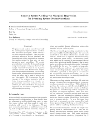
Figure 1, graphs a histogram of the ratio of smooth
sparse coding Fisher score over standard sparse coding
Fisher score R(d) = F1(d)/F2(d) for 15-scene dataset
(left) and Youtube dataset (right). Both histograms
demonstrate the improved discriminatory power of
smooth sparse coding over regular sparse coding.
7. Semi-supervised smooth sparse
coding
One of the primary difficulties in some image classifica-
tion tasks is the lack of availability of labeled data and
in some cases, both labeled and unlabeled data (for
particular domains). This motivated semi-supervised
learning and transfer learning without labels (Raina
et al., 2007) respectively. The motivation for such ap-
proaches is that data from a related domain might
have some visual patterns that might be similar to the
problem at hand. Hence, learning a high-level dictio-
nary based on data from a different domains aids the
classification task of interest.
We propose that the smooth sparse coding approach
might be useful in this setting. The motivation is as

0.8 1 1.2 1.4 1.6 1.8 2
0
50
100
150
200
250
300
350
400
450
500
R(d)
0.8 0.9 1 1.1 1.2 1.3 1.4 1.5
0
100
200
300
400
500
600
700
R(d)
Figure 1. Comparison between the histograms of Fisher discriminant score realized by sparse coding and smooth sparse
coding. The images represent the histogram of the ratio of smooth sparse coding Fisher score over standard sparse coding
Fisher score (left: image data set; right: video). A value greater than 1 implies that smooth sparse coding is more
discriminatory.
follows: in semi-supervised, typically not all samples
from a different data set might be useful for the task at
hand. Using smooth sparse coding, one can weigh the
useful points more than the other points (the weights
being calculated based on feature/time similarity ker-
nel) to obtain better dictionaries and sparse represen-
tations. Other approach to handle a lower number
of labeled samples include collaborative modeling or
multi-task approaches which impose a shared struc-
ture on the codes for several tasks and use data from
all the tasks simultaneously, for example group sparse
coding (Bengio et al., 2009). The proposed approach
provides an alternative when such collaborative mod-
eling assumptions do not hold, by using relevant unla-
beled data samples that might help the task at hand
via appropriate weighting.
We now describe an experiment that examines the pro-
posed smoothed sparse coding approach in the con-
text of semi-supervised dictionary learning. We use
data from both CMU multi-pie dataset (session 1) and
faces-on-tv dataset (treated as frames) to learn a dic-
tionary using a feature similarity kernel. We follow the
same procedure described in the previous experiments
to construct the dictionary. In the test stage we use
the obtained dictionary for coding data from sessions
2, 3, 4 of CMU-multipie data set, using smooth sparse
coding. Note that semi-supervision was used only in
the dictionary learning stage (the classification stage
used supervised SVM).
Table 5 shows the test set error rate and compares it
to standard sparse coding and LLC (Yu et al., 2009).
Smooth sparse coding achieves significantly lower test
error rate than the two alternative techniques. We con-
clude that the smoothing approach described in this
paper may be useful in cases where there is a small set
of labeled data, such as semisupervised learning and
transfer learning.
Method SC LLC SSC-tricube
Test errror 6.345 6.003 4.975
Table 5. Semi-supervised learning test set error: Dictio-
nary learned from both CMU multi-pie and faces-on-tv
data set using feature similarity kernel, used to construct
sparse codes for CMU multipie data set.
8. Discussion and Future work
We proposed a simple framework for incorporating
similarity in feature space and space or time into sparse
coding. We also propose in this paper modifying
sparse coding by replacing the lasso optimization stage
by marginal regression and adding a constraint to en-
force incoherent dictionaries. The resulting algorithm
is significantly faster (speedup of about two-orders of
magnitude over standard sparse coding). This facili-
tates scaling up the sparse coding framework to large
dictionaries, an area which is usually restricted due to
intractable computation.
This works leads to several interesting follow-up work.
On the theoritical side: (i) local convergence of Lasso-
based sparse coding has been analyzed in (Jenatton
et al., 2012)- preliminary examination suggests that
the proposed marginal-regression based sparse coding
algorithm might be more favorable for the local con-
vergence analysis and (ii) it is also interesting to ex-
plore tighter generalization error bounds by directly
analyzing the solutions of the marginal regression iter-
ative algorithm. Methodologically, it is interesting to
explore: (i) using an adaptive or non-constant kernel
bandwidth to get higher accuracy, and (iv) alternative
incoherence constraints that may lead to easier opti-
mization and scaling up.

References
Bartlett, P.L., Bousquet, O., and Mendelson, S. Local
rademacher complexities. The Annals of Statistics,
2005.
Bengio, S., Pereira, F., Singer, Y., and Strelow, D.
Group sparse coding. In NIPS, 2009.
Bertsekas, D. On the goldstein-levitin-polyak gradient
projection method. IEEE Transactions on Auto-
matic Control, 1976.
Bronstein, A., Sprechmann, P., and Sapiro, G. Learn-
ing efficient structured sparse models. ICML, 2012.
Devroye, L. and Lugosi, G. Combinatorial methods in
density estimation. 2001.
Fan, J. and Lv, J. Sure independence screening
for ultrahigh dimensional feature space. JRSS:
B(Statistical Methodology), 2008.
Genovese, C. R., Jin, J., Wasserman, L., and Yao, Z.
A comparison of the lasso and marginal regression.
JMLR, 2012.
Hastie, T. and Loader, C. Local regression: Automatic
kernel carpentry. Statistical Science, pp. 120–129,
1993.
Jenatton, R., Mairal, J., Obozinski, G., and Bach, F.
Proximal methods for sparse hierarchical dictionary
learning. ICML, 2010.
Jenatton, R., Gribonval, R., and Bach, F. Lo-
cal stability and robustness of sparse dictionary
learning in the presence of noise. arXiv preprint
arXiv:1210.0685, 2012.
Kläser, A., Marszalek, M., and Schmid, C. A spatio-
temporal descriptor based on 3d-gradients. In
BMVC, 2008.
Lee, H., Battle, A., Raina, R., and Ng, A.Y. Efficient
sparse coding algorithms. In NIPS, 2007.
Liu, J., Luo, J., and Shah, M. Recognizing realistic
actions from videos in the wild. In CVPR, 2009.
Loader, C. Local regression and likelihood. Springer
Verlag, 1999.
Lowe, D. G. Object recognition from local scale-
invariant features. CVPR, 1999.
Magnus, J. R. and Neudecker, H. Matrix differential
calculus with applications in statistics and econo-
metrics. 1988.
Meier, L. and Bühlmann, P. Smoothing l1-penalized
estimators for high-dimensional time-course data.
Electronic Journal of Statistics, 2007.
Raina, R., Battle, A., Lee, H., Packer, B., and Ng,
A.Y. Self-taught learning: transfer learning from
unlabeled data. In ICML, 2007.
Ramırez, I., Lecumberry, F., and Sapiro, G. Sparse
modeling with universal priors and learned incoher-
ent dictionaries. Tech Report, IMA, University of
Minnesota, 2009.
Sigg, C. D., Dikk, T., and Buhmann, J. M. Learn-
ing dictionaries with bounded self-coherence. IEEE
Transactions on Signal Processing, 2012.
Solodov, M. V. Convergence analysis of perturbed fea-
sible descent methods. Journal of Optimization The-
ory and Applications, 1997.
Tropp, J.A. Greed is good: Algorithmic results for
sparse approximation. Information Theory, IEEE,
2004.
Vainsencher, D., Mannor, S., and Bruckstein, A.M.
The sample complexity of dictionary learning.
JMLR, 2011.
Wang, H., Ullah, M.M., Klaser, A., Laptev, I., and
Schmid, C. Evaluation of local spatio-temporal fea-
tures for action recognition. In BMVC, 2009.
Yang, J., Yu, K., and Huang, T. Supervised
translation-invariant sparse coding. In CVPR, 2010.
Yu, K., Zhang, T., and Gong, Y. Nonlinear learning
using local coordinate coding. NIPS, 2009.
Yu, K., Lin, Y., and Lafferty, J. Learning image repre-
sentations from the pixel level via hierarchical sparse
coding. In CVPR, 2011.
Zangwill, W.I. Nonlinear programming: a unified ap-
proach. 1969.

ssc_icml13

Recommended

Recommended

More Related Content

What's hot

What's hot (19)

Similar to ssc_icml13

Similar to ssc_icml13 (20)

ssc_icml13