Engineering mechanics iii-lecture_notes_of_meen-321_kinematics_of_machinery_handouts_to_students-libre

MECHANICAL ENGINEERING DEPARTMENT, ERITREA INSTITUTE OF TECHNOLOGY.
Prepared by Kiran Kumar.K, Lecturer. (E-mail:- kiranmedesign@gmail.com)
1
MEEN 321 ENGINEERING MECHANICS-III (MECHANISMS) 3 Cr.
Unit:I Simple Mechanism
1.1 Introduction
Mechanics: It is that branch of scientific analysis which deals with motion, time and
force.
Kinematics is the study of motion, without considering the forces which produce that
motion. Kinematics of machines deals with the study of the relative motion of machine
parts. It involves the study of position, displacement, velocity and acceleration of
machine parts.
Dynamics of machines involves the study of forces acting on the machine parts and the
motions resulting from these forces.
Plane motion: A body has plane motion, if all its points move in planes which are
parallel to some reference plane. A body with plane motion will have only three degrees
of freedom. I.e., linear along two axes parallel to the reference plane and
rotational/angular about the axis perpendicular to the reference plane. (eg. linear along X
and Z and rotational about Y.)The reference plane is called plane of motion. Plane motion
can be of three types. 1) Translation 2) rotation and 3) combination of translation and
rotation.
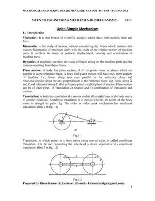
Translation: A body has translation if it moves so that all straight lines in the body move
to parallel positions. Rectilinear translation is a motion wherein all points of the body
move in straight lie paths. Eg. The slider in slider crank mechanism has rectilinear
translation. (link 4 in fig.1.1)
Fig.1.1
Translation, in which points in a body move along curved paths, is called curvilinear
translation. The tie rod connecting the wheels of a steam locomotive has curvilinear
translation. (link 3 in fig.1.2)
Fig.1.2

2
Rotation: In rotation, all points in a body remain at fixed distances from a line which is
perpendicular to the plane of rotation. This line is the axis of rotation and points in the
body describe circular paths about it. (Eg. link 2 in Fig.1.1 and links 2 & 4 in Fig.1.2)
Translation and rotation: It is the combination of both translation and rotation which is
exhibited by many machine parts. (Eg. link 3 in Fig.1.1)
1.2 Kinematic link (or) element
A machine part or a component of a mechanism is called a kinematic link or simply a
link. A link is assumed to be completely rigid, or under the action of forces it does not
suffer any deformation, signifying that the distance between any two points on it remains
constant. Although all real machine parts are flexible to some degree, it is common
practice to assume that deflections are negligible and parts are rigid when analyzing a
machine’s kinematic performance.
1.3 Types of link
(a) Based on number of elements of link:
Binary link: Link which is connected to other links at two points. (Fig.1.3 a)
Ternary link: Link which is connected to other links at three points. (Fig.1.3 b)
Quaternary link: Link which is connected to other links at four points. (Fig1.3 c)
Fig.1.3
(a) Based on type of structural behavior:
Sometimes, a machine member may possess one-way rigidity and is capable of
transmitting the force in one direction with negligible deformation. Examples are (a)
chains, belts and ropes which are resistant to tensile forces, and (b) fluids which are
resistant to compressive forces and are used as links in hydraulic presses, brakes and
jacks. In order to transmit motion, the driver and the follower may be connected by the
following three types of links:
1. Rigid link. A rigid link is one which does not undergo any deformation while
transmitting motion. Strictly speaking, rigid links do not exist. However, as the
deformation of a connecting rod, crank etc. of a reciprocating steam engine is not
appreciable, they can be considered as rigid links.
2. Flexible link. A flexible link is one which is partly deformed in a manner not to affect
the transmission of motion. For example, belts, ropes, chains and wires are flexible links
and transmit tensile forces only.

3
3. Fluid link. A fluid link is one which is formed by having a fluid in a receptacle and the
motion is transmitted through the fluid by pressure or compression only, as in the case of
hydraulic presses, jacks and brakes.
1.4 Structure
It is an assemblage of a number of resistant bodies (known as members) having no
relative motion between them and meant for carrying loads having straining action. A
railway bridge, a roof truss, machine frames etc., are the examples of a structure.
Machine: A machine is a mechanism or collection of mechanisms, which transmit force
from the source of power to the resistance to be overcome. Though all machines are
mechanisms, all mechanisms are not machines. Many instruments are mechanisms but
are not machines, because they do no useful work nor do they transform energy.
1.5 Difference between structure & machine
The following differences between a machine and a structure are important from the
subject point of view:
1. The parts of a machine move relative to one another, whereas the members of a
structure do not move relative to one another.
2. A machine transforms the available energy into some useful work, whereas in a
structure no energy is transformed into useful work.
3. The links of a machine may transmit both power and motion, while the members of a
structure transmits forces only.
Comparison of Mechanism, Machine and Structure
Mechanism Machine Structure
1. There is relative
motion between the parts
of a mechanism
Relative motion exists
between parts of a
machine.
There is no relative
motion between the
members of a structure. It
is rigid as a whole.
2. A mechanism modifies
and transmits motion.
A machine consists of
one or more mechanisms
and hence transforms
motion
A structure does not
transform motion.
3. A mechanism does not
transmit forces and does
not do work
A machine modifies
energy or do some work
A structure does not do
work. It only transmits
forces.
4. Mechanisms are dealt
with in kinematics.
Machines are dealt with
in kinetics.
Structures are dealt with
in statics.

4
1.6 Kinematic pair
The two links or elements of a machine, when in contact with each other, are said to form
a pair. If the relative motion between them is completely or successfully constrained (i.e.
in a definite direction), the pair is known as kinematic pair.
1.7 Types of constrained motion
Constrained motion: In a kinematic pair, if one element has got only one definite
motion relative to the other, then the motion is called constrained motion.
(a) Completely constrained motion. If the constrained motion is achieved by the pairing
elements themselves, then it is called completely constrained motion.
completely constrained motion
(b) Successfully constrained motion. If constrained motion is not achieved by the
pairing elements themselves, but by some other means, then, it is called successfully
constrained motion. Eg. Foot step bearing, where shaft is constrained from moving
upwards, by its self weight.
(c) Incompletely constrained motion. When relative motion between pairing elements
takes place in more than one direction, it is called incompletely constrained motion. Eg.
Shaft in a circular hole.
Foot strep bearing Incompletely constrained motion

5
1.8 Classification of kinematic pair
The kinematic pairs may be classified according to the following considerations :
(i) Based on nature of contact between elements:
(a) Lower pair. If the joint by which two members are connected has surface contact,
the pair is known as lower pair. Eg. pin joints, shaft rotating in bush, slider in slider
crank mechanism.
Lower pairs
(b) Higher pair. If the contact between the pairing elements takes place at a point or
along a line, such as in a ball bearing or between two gear teeth in contact, it is
known as a higher pair.
Higher pairs
(ii) Based on relative motion between pairing elements:
(a) Siding pair. Sliding pair is constituted by two elements so connected that one is
constrained to have a sliding motion relative to the other. DOF = 1
(b) Turning pair (revolute pair). When connections of the two elements are such that
only a constrained motion of rotation of one element with respect to the other is
possible, the pair constitutes a turning pair. DOF = 1
(c) Cylindrical pair. If the relative motion between the pairing elements is the
combination of turning and sliding, then it is called as cylindrical pair. DOF = 2

6
Sliding pair Turning pair
Cylindrical pair
(d) Rolling pair. When the pairing elements have rolling contact, the pair formed is
called rolling pair. Eg. Bearings, Belt and pulley. DOF = 1
Ball bearing Belt and pulley
(e) Spherical pair. A spherical pair will have surface contact and three degrees of
freedom. Eg. Ball and socket joint. DOF = 3
(f) Helical pair or screw pair. When the nature of contact between the elements of a
pair is such that one element can turn about the other by screw threads, it is known
as screw pair. Eg. Nut and bolt. DOF = 1
Ball and socket joint Screw pair

7
Pair Pair variable
Degree of
freedom
Relative motion
Revolute  1 Circular
Prism S 1 Linear
Screw or S 1 Helical
Cylinder and S 2 Cylindrical
Sphere and  3 Spherical
Flat x and Y 3 Planar
(a) Sliding pair (prismatic pair) eg. piston and cylinder, crosshead and slides, tail stock
on lathe bed.
(b) Turning pair (Revolute pair): eg: cycle wheel on axle, lathe spindle in head stock.
(c) Cylindrical pair: eg. shaft turning in journal bearing.
(d) Screw pair (Helical pair): eg. bolt and nut, lead screw of lathe with nut, screw jack.
(e) Spherical pair: eg. penholder on stand, castor balls.
(f) Flat pair: Seldom found in mechanisms.
(iii) Based on the nature of mechanical constraint.
(a) Closed pair. Elements of pairs held together mechanically due to their geometry
constitute a closed pair. They are also called form-closed or self-closed pair.
(b) Unclosed or force closed pair. Elements of pairs held together by the action of
external forces constitute unclosed or force closed pair .Eg. Cam and follower.
Closed pair Force closed pair (cam & follower)

8
1.9 Kinematic chain
When the kinematic pairs are coupled in such a way that the last link is joined to the first
link to transmit definite motion (i.e. completely or successfully constrained motion), it is
called a kinematic chain. Relation between the number of links (l) and the number of
joints ( j ) which constitute a kinematic chain is given by the expression :
Let us apply the above equations to the following cases to determine whether each of
them is a kinematic chain or not.
If, for a particular position of a link of the chain, the positions of each of the other links
of the chain cannot be predicted, then it is called as unconstrained kinematic chain and
it is not mechanism.

9
The above one is constrained kinematic chain.
1.10 types of joints in chain
The following types of joints are usually found in a chain:
1. Binary joint. When two links are joined at the same connection, the joint is known as binary
joint.
2. Ternary joint. When three links are joined at the same connection, the joint is known as ternary
joint.
3. Quaternary joint. When four links are joined at the same connection, the joint is called a
quaternary joint. It is equivalent to three binary joints.
1.11 Mechanism
When one of the links of a kinematic chain is fixed, the chain is known as mechanism.
A mechanism with four links is known as simple mechanism, and the mechanism with
more than four links is known as compound mechanism. When a mechanism is required
to transmit power or to do some particular type of work, it then becomes a machine.
A mechanism is a constrained kinematic chain. This means that the motion of any one
link in the kinematic chain will give a definite and predictable motion relative to each of
the others. Usually one of the links of the kinematic chain is fixed in a mechanism.

10
Slider crank and four bar mechanisms.
1.12 Number of degrees of freedom for plane mechanism
Degrees of freedom/mobility of a mechanism: The number of independent input
parameters (or pair variables) that are needed to determine the position of all the links of
the mechanism with respect to the fixed link is termed its degrees of freedom.
Degrees of freedom (DOF) is the number of independent coordinates required to describe
the position of a body in space. A free body in space can have six degrees of freedom.
I.e., linear positions along x, y and z axes and rotational/angular positions with respect to
x, y and z axes. In a kinematic pair, depending on the constraints imposed on the motion,
the links may loose some of the six degrees of freedom.
Planar mechanisms: When all the links of a mechanism have plane motion, it is called
as a planar mechanism. All the links in a planar mechanism move in planes parallel to the
reference plane.
Serial Mechanisms (Manipulators): Early manipulators were work holding devices in
manufacturing operations so that the work piece could be manipulated or brought to
different orientations with respect to the tool head. Welding robots of the auto industry
and assembly robots of IC manufacture are examples.
1.13 Application of kutzbach criterion to Plane mechanisms
F = 3 (n–1) – 2l – h
Where n=number of links; l= number of lower joints (or) pairs and h= number of higher
pairs (or) joints
This is called the Kutzbach criterion for the mobility of a planar mechanism.

11
Examples of determination of degrees of freedom of planar mechanisms:
(i)
F = 3(n-1)-2l-h
Here, n2 = 4, n = 4, l = 4 and h = 0.
F = 3(4-1)-2(4) = 1
I.e., one input to any one link will result in
definite motion of all the links.
(ii)
F = 3(n-1)-2l-h
Here, n2 = 5, n = 5, l = 5 and h = 0.
F = 3(5-1)-2(5) = 2
I.e., two inputs to any two links are
required to yield definite motions in all the
links.
(iii)
F = 3(n-1)-2l-h
Here, n2 = 4, n3 =2, n = 6, l = 7 and h = 0.
F = 3(6-1)-2(7) = 1
I.e., one input to any one link will result in
definite motion of all the links.

12
1.15 Inversion of Mechanism
A mechanism is one in which one of the links of a kinematic chain is fixed. Different
mechanisms can be obtained by fixing different links of the same kinematic chain. These
are called as inversions of the mechanism.
1.16 Inversions of Four Bar Chain
One of the most useful and most common mechanisms is the four-bar linkage. In this
mechanism, the link which can make complete rotation is known as crank (link 2). The
link which oscillates is known as rocker or lever (link 4). And the link connecting these
two is known as coupler (link 3). Link 1 is the frame.

13
Inversions:
Fig.1.23 Inversions of four bar chain.
Crank-rocker mechanism: In this mechanism, either link 1 or link 3 is fixed. Link 2
(crank) rotates completely and link 4 (rocker) oscillates. It is similar to (a) or (b) of
fig.1.23.
Fig.1.24
Beam engine (crank and lever mechanism).
A part of the mechanism of a beam engine (also known as crank and lever mechanism)
which consists of four links, is shown in Fig. In this mechanism, when the crank rotates
about the fixed centre A, the lever oscillates about a fixed centre D. The end E of the
lever CDE is connected to a piston rod which reciprocates due to the rotation of the
crank. In other words, the purpose of this mechanism is to convert rotary motion into
reciprocating motion.

14
Double crank mechanism (Coupling rod of locomotive). This is one type of drag link
mechanism, where, links 1& 3 are equal and parallel and links 2 & 4 are equal and
parallel.
The mechanism of a coupling rod of a locomotive (also known as double crank
mechanism) which consists of four links in the fig. in this mechanism, the links AD and
BC (having equal length) act as cranks and are connected to the respective wheels. The
link CD acts as a coupling rod and the link AB is fixed in order to maintain a constant
centre to centre distance between them. This mechanism is meant for transmitting rotary
motion from one wheel to the other wheel.
Fig.1.26
Double rocker mechanism. In this mechanism, link 4 is fixed. Link 2 makes complete
rotation, whereas links 3 & 4 oscillate (Fig.1.23d)
Coupler Curves: The link connecting the driving crank with the follower crank in a
four bar linkage is called the coupler. Similarly, in the case of a single slider crank
mechanism the connecting rod is the coupler. During the motion of the mechanism any
point attached to the coupler generates some path with respect to the fixed link. This path
is called the coupler curve. The point, which generates the path is variously called the
coupler point, trace point, tracing point, or tracer point.
An example of the coupler curves generated by different coupler points is given
in figure below. Mechanisms can be designed to generate any curve.

15
1.17 Inversions of Single Slider Chain
Slider crank chain: This is a kinematic chain having four links. It has one sliding pair
and three turning pairs. Link 2 has rotary motion and is called crank. Link 3 has got
combined rotary and reciprocating motion and is called connecting rod. Link 4 has
reciprocating motion and is called slider. Link 1 is frame (fixed). This mechanism is used
to convert rotary motion to reciprocating and vice versa.
Fig1.27
Inversions of slider crank chain
Inversions of slider crank mechanism is obtained by fixing links 2, 3 and 4.
(a) crank fixed (b) connecting rod fixed (c) slider fixed
Fig.1.28

16
Rotary engine – Inversion of slider crank mechanism. (Crank fixed)
Sometimes back, rotary internal combustion engines were used in aviation. But now-a-
days gas turbines are used in its place. It consists of seven cylinders in one plane and all
revolves about fixed centre D, as shown in Fig., while the crank (link 2) is fixed. In this
mechanism, when the connecting rod (link4) rotates, the piston (link 3) reciprocates
inside the cylinders forming link 1.
Fig.1.29
Quick return motion mechanisms.
Quick return mechanisms are used in machine tools such as shapers and power driven
saws for the purpose of giving the reciprocating cutting tool a slow cutting stroke and a
quick return stroke with a constant angular velocity of the driving crank.
Whitworth quick return motion mechanism–Inversion of slider crank mechanism.
This mechanism is mostly used in shaping and slotting machines. In this mechanism, the
link CD (link 2) forming the turning pair is fixed, as shown in Fig. The link 2
corresponds to a crank in a reciprocating steam engine. The driving crank CA (link 3)
rotates at a uniform angular speed. The slider (link 4) attached to the crank pin at A slides
along the slotted bar PA(link 1) which oscillates at a pivoted point D. The connecting rod
PR carries the ram at R to which a cutting tool is fixed. The motion of the tool is
constrained along the line RD produced, i.e. along a line passing through D and
perpendicular to CD.
Fig.1.30

17
When the driving crank CAmoves from the position CA1 to CA2 (or the link DP from
the position DP1 to DP2) through an angle αin the clockwise direction, the tool moves
from the left hand end of its stroke to the right hand end through a distance 2 PD.
Now when the driving crank moves from the position CA2 to CA1 (or the link DP from
DP2 to DP1 ) through an angle βin the clockwise direction, the tool moves back from
right hand end of its stroke to the left hand end.
A little consideration will show that the time taken during the left to right movement of
the ram (i.e. during forward or cutting stroke) will be equal to the time taken by the
driving crank to move from CA1 to CA2. Similarly, the time taken during the right to left
movement of the ram (or during the idle or return stroke) will be equal to the time taken
by the driving crank to move from CA2 to CA1.
Since the crank link CArotates at uniform angular velocity therefore time taken during
the cutting stroke (or forward stroke) is more than the time taken during the return stroke.
In other words, the mean speed of the ram during cutting stroke is less than the mean
speed during the return stroke.
The ratio between the time taken during the cutting and return strokes is given by
Crank and slotted lever quick return motion mechanism – Inversion of slider crank
mechanism (connecting rod fixed).
This mechanism is mostly used in shaping machines, slotting machines and in rotary
internal combustion engines. In this mechanism, the link AC (i.e. link 3) forming the
turning pair is fixed, as shown in Fig. The link 3 corresponds to the connecting rod of a
reciprocating steam engine. The driving crank CB revolves with uniform angular speed
about the fixed centre C. A sliding block attached to the crank pin at B slides along the
slotted bar AP and thus causes AP to oscillate about the pivoted point A. A short link PR
transmits the motion from AP to the ram which carries the tool and reciprocates along the
line of stroke R1R2. The line of stroke of the ram (i.e. R1R2) is perpendicular to AC
produced.
We see that the angle βmade by the forward or cutting stroke is greater than the angle
αdescribed by the return stroke. Since the crank rotates with uniform angular speed,
therefore the return stroke iscompleted within shorter time. Thus it is called quick return
motion mechanism.
In the extreme positions, AP1 and AP2 are tangential to the circle and the cutting tool is
at the end of the stroke. The forward or cutting stroke occurs when the crank rotates from
the position CB1 to CB2 (or through an angle β) in the clockwise direction. The return
stroke occurs when the crank rotates from the position CB2 to CB1 (or through angle α)
in the clockwise direction. Since the crank has uniform angular speed, therefore,

18
Oscillating cylinder engine–Inversion of slider crank mechanism (connecting rod
fixed).
The arrangement of oscillating cylinder engine mechanism, as shown in Fig., is used to
convert reciprocating motion into rotary motion. In this mechanism, the link 3 forming
the turning pair is fixed. The link 3 corresponds to the connecting rod of a reciprocating
steam engine mechanism. When the crank (link2) rotates, the piston attached to piston
rod (link 1) reciprocates and the cylinder (link 4) oscillates about a pin pivoted to the
fixed link at A.

19
Pendulum pump or bull engine–Inversion of slider crank mechanism (slider fixed).
In this mechanism, the inversion is obtained by fixing the cylinder or link 4 (i.e. sliding
pair), as shown in Fig. In this case, when the crank (link 2) rotates, the connecting rod
(link 3) oscillates about a pin pivoted to the fixed link 4 at A and the piston attached to
the piston rod (link 1) reciprocates. The duplex pump which is used to supply feed water
to boilers have two pistons attached to link 1, as shown in Fig.
1.18 Inversions of Double slider Crank Chain
Double slider crank chain: It is a kinematic chain consisting of two turning pairs and
two sliding pairs. With this chain three inversions are possible. The link between the
revolute pairs can be fixed, and one such mechanism based on this inversion is the
Oldham’s coupling. When the link with one revolute pair and one prismatic pair is fixed
the inversion results in the Scotch-yoke mechanism. The third case when the link with
two prismatic pairs is fixed has the Elliptic or Ellipse trammel as an application.
Inversions:
Scotch –Yoke mechanism: This mechanism is used for converting rotary motion into
reciprocating motion. The inversion is obtained by fixing either link 1 or link 3. The
figure shows the mechanism with link 1 fixed. When link 2, which corresponds to the
crank, rotates about B as centre, the link 4 reciprocates. Link 4 has a slot in which the
slider A (link 3) slides, and the fixed link 1 guides this frame.
Fig.1.34

20
Elliptical trammel: This is a device which is used for generating an elliptical profile.
In this the link 4 is fixed. It is a slotted frame with two slots at right angles in
which two die blocks slide along the slots. These are the links 1 and 3. The link AB (link
2) is a bar which forms turning pairs with links 1 and 3.
When the links 1 and 3 slide along their respective grooves any point on link 2,
such as P traces out an ellipse on the surface of link 4 with AP and BP the semi-major
and semi-minor axes respectively of the ellipse.
Fig.1.35
Oldham coupling: This is an inversion of double slider crank mechanism, which is used
to connect two parallel shafts, whose axes are offset by a small amount. An Oldham’s
coupling is used for connecting two parallel shafts whose axes are at a small distance
apart. This coupling ensures that if one shaft rotates, the other shaft also rotates at the
same speed. This inversion is obtained by fixing the link 2. The shafts have two flanges
(link 1 and link 3). The links 1 and 3 form turning pairs with the frame link 2. Each
flange is identical in form and has a single slot cut diametrically across each face. The
intermediate piece (link 4) which is a circular disc with a tongue passing diametrically
across each face and the two tongues are set at right angles to each other so that each
tongue fits into its corresponding slot in one of the flanges. The tongues are sliding fit in
their slots. So long as the shafts remain parallel to each other their distance apart may
vary while the shafts are in motion without affecting the transmission of uniform motion
from one shaft to the other.
Fig.1.36

21
Unit:II VELOCITY AND ACCELERATION ANALYSIS OF
MECHANISMS
In this chapter, we shall discuss the relative velocity method for determining the velocity
of different points in the mechanism. The study of velocity analysis is very important for
determining the acceleration of points in the mechanisms.
Kinematics deals with study of relative motion between the various parts of the machines.
Kinematics does not involve study of forces. Thus motion leads study of displacement,
velocity and acceleration of a part of the machine. As dynamic forces are a function of
acceleration and acceleration is a function of velocities, study of velocity and acceleration
will be useful in the design of mechanism of a machine. The mechanism will be
represented by a line diagram which is known as configuration diagram. The analysis
can be carried out both by graphical method as well as analytical method.
Displacement: All particles of a body move in parallel planes and travel by same distance
is known, linear displacement and is denoted by ‘x’. A body rotating about a fired point
in such a way that all particular move in circular path angular displacement and is
denoted by ‘’.
Velocity: Rate of change of displacement is velocity. Velocity can be linear
velocity of angular velocity.
Linear velocity is Rate of change of linear displacement= V =
dt
dx
Angular velocity is Rate of change of angular displacement =  =
dt
d
Relation between linear velocity and angular velocity.
x = r
dt
dx
= r
dt
d
V = r
 =
dt
d
Acceleration: Rate of change of velocity
f = 2
2
dt
xd
dt
dv
 Linear Acceleration (Rate of change of linear velocity)
Thirdly  = 2
2
dt
d
dt
d 
 Angular Acceleration (Rate of change of angular velocity)
Absolute velocity: Velocity of a point with respect to a fixed point (zero velocity point).
Vao2 = 2 x r
Vao2 = 2 x O2 A
Ex: Vao2 is called absolute velocity.
O2
2
A

22
2.1 motion of a link
Consider two points A and B on a rigid link AB, as shown in Fig. (a). Let one of the extremities
(B) of the link move relative to A, in a clockwise direction. Since the distance from A to B
remains the same, therefore there can be no relative motion between A and B, along the line AB.
It is thus obvious, that the relative motion of B with respect to A must be perpendicular to AB.
Hence velocity of any point on a link with respect to another point on the same link is
always perpendicular to the line joining these points on the configuration (or space)
diagram.
The relative velocity of B with respect to A(i.e. vBA) is represented by the vector ab and is
perpendicular to the line AB as shown in Fig. (b).
From the above two equations
Thus, we see from above equation that the point c on the vector ab divides it in the same ratio as
C divides the link AB.
Note: The relative velocity of Awith respect to B is represented by ba, although A may be a fixed
point. The motion between A and B is only relative. Moreover, it is immaterial whether the link
moves about Ain a clockwise direction or about B in a clockwise direction.
2.2 Rubbing Velocity at a Pin Joint

23
The links in a mechanism are mostly connected by means of pin joints. The rubbing velocity is
defined as the algebraic sum between the angular velocities of the two links which are
connected by pin joints, multiplied by the radius of the pin.
Consider two links OAand OB connected by a pin joint at O as shown in Fig.
Let
ω1 = Angular velocity of the link OAor the angular velocity of the point Awith respect to O
ω2 = Angular velocity of the link OB or the angular velocity of the point B with respect to O, and
r = Radius of the pin.
According to the definition,
Rubbing velocity at the pin joint O is given by the formula
=(ω1-ω2)*r , if the links move in the same direction
= (ω1+ω2)*r, if the links move in the opposite direction
where ω1 = angular velocity of link 1
ω2 = angular velocity of link 2
r = radius of the pin
Note : When the pin connects one sliding member and the other turning member, the angular
velocity of the sliding member is zero. In such cases,
Rubbing velocity at the pin joint = ωr
where ω=Angular velocity of the turning member, and
r = Radius of the pin.
Acceleration in mechanisms
2.3 acceleration of a mechanism (Introduction)
We have discussed in the previous chapter the velocities of various points in the mechanisms.
Now we shall discuss the acceleration of points in the mechanisms. The acceleration analysis
plays a very important role in the development of machines and mechanisms.
2.4 acceleration diagram for a link
Consider two points Aand B on a rigid link as shown in Fig. (a). Let the point B moves with respect to A,
with an angular velocity of ωrad/s and let αrad/s
2
be the angular acceleration of the link AB.

24
We have already discussed that acceleration of a particle whose velocity changes both in
magnitude and direction at any instant has the following two components:
1. The centripetal or radial component, which is perpendicular to the velocity of the particle at
the given instant.
2. The tangential component, which is parallel to the velocity of the particle at the given instant.
Thus for a link AB, the velocity of point B with respect to A(i.e. vBA) is perpendicular to the link
AB as shown in Fig.(a). Since the point B moves with respect to A with an angular velocity of ω
rad/s, therefore centripetal or radial component of the acceleration of B with respect to A,
This radial component of acceleration acts perpendicular to the velocity vBA, In other words, it acts parallel
to the link AB.
We know that tangential component of the acceleration of B with respect to A,
This tangential component of acceleration acts parallel to the velocity vBA. In other words, it acts
perpendicular to the link AB.
In order to draw the acceleration diagram for a link AB, as shown in Fig. (b), from any point b',
draw vector b'x parallel to BA to represent the radial component of acceleration of B with respect
to A i.e. from point x draw vector xa' perpendicular to B A to represent the tangential
component of acceleration of B with respect to A i.e. . Join b' a'. The vector b' a' (known as
acceleration image of the link AB) represents the total acceleration of B with respect to A (i.e.
aBA) and it is the vector sum of radial component and tangential component of
acceleration.
Exercise Problems:
1. In a four bar chain ABCD link AD is fixed and in 15 cm long. The crank AB is 4 cm
long rotates at 180 rpm (cw) while link CD rotates about D is 8 cm long BC = AD
and BAD| = 60o
. Find angular velocity of link CD.
Configuration Diagram
60o
ωBA
A D
B
C
15 cm
15 cm
8 cm

25
Velocity vector diagram
Vb = r = ba x AB = 4x
60
120x2π
= 50.24 cm/sec
Choose a suitable scale
1 cm = 20 m/s = ab
Vcb = bc
Vc = dc = 38 cm/sec = Vcd
We know that V =ω R
Vcd = CD x CD
ωcD = 75.4
8
38Vcd

CD
rad/sec (cw)
2. In a crank and slotted lever mechanism crank rotates of 300 rpm in a counter
clockwise direction. Find
(i) Angular velocity of connecting rod and
(ii) Velocity of slider.
Configuration diagram
Step 1: Determine the magnitude and velocity of point A with respect to 0,
VA = O1A x O2A = 60x
60
300x2π
= 600  mm/sec
Step 2: Choose a suitable scale to draw velocity vector diagram.
r
to CD
r
to BC
r
to AB
a, d
b
c Vcb
60 mm
45o
A
B
150 mm

26
Vab = ab=1300mm/sec
ba = 66.8
150
1300

BA
Vba
rad/sec
Vb = obvelocity of slider
Note: Velocity of slider is along the line of sliding.
3. In a four bar mechanism, the dimensions of the links are as given below:
AB = 50 mm, BC = 66 mm
CD = 56 mm and AD = 100 mm
At a given instant when o
60DAB|  the angular velocity of link AB is 10.5
rad/sec in CCW direction.
Determine,
i) Velocity of point C
ii) Velocity of point E on link BC when BE = 40 mm
iii) The angular velocity of link BC and CD
iv) The velocity of an offset point F on link BC, if BF = 45 mm, CF = 30
mm and BCF is read clockwise.
v) The velocity of an offset point G on link CD, if CG = 24 mm, DG = 44
mm and DCG is read clockwise.
vi) The velocity of rubbing of pins A, B, C and D. The ratio of the pins
are 30 mm, 40 mm, 25 mm and 35 mm respectively.
Solution:
Step -1: Construct the configuration diagram selecting a suitable scale.
Scale: 1 cm = 20 mm
O
Vaa
b
r
to AB r
to OA
Along sides B

27
Step – 2: Given the angular velocity of link AB and its direction of rotation determine
velocity of point with respect to A (A is fixed hence, it is zero velocity point).
Vba = BA x BA
= 10.5 x 0.05 = 0.525 m/s
Step – 3: To draw velocity vector diagram choose a suitable scale, say 1 cm = 0.2 m/s.
 First locate zero velocity points.
 Draw a line r
to link AB in the direction of rotation of link AB (CCW) equal to
0.525 m/s.
 From b draw a line r
to BC and from d. Draw d line r
to CD to interest at C.
 Vcb is given vector bc Vbc = 0.44 m/s
 Vcd is given vector dc Vcd = 0.39 m/s
Step – 4: To determine velocity of point E (Absolute velocity) on link BC, first locate the
position of point E on velocity vector diagram. This can be done by taking corresponding
ratios of lengths of links to vector distance i.e.
BC
BE
bc
be

 be =
BC
BE
x Vcb =
066.0
04.0
x 0.44 = 0.24 m/s
60o
A D
B
C
F
G
C
f
Ved
a, d
e, g
Vba = 0.525 m/s
b

28
Join e on velocity vector diagram to zero velocity points a, d / vector de = Ve =
0.415 m/s.
Step 5: To determine angular velocity of links BC and CD, we know Vbc and Vcd.
 Vbc =ω BC x BC
 ωBC = )(./6.6
066.0
44.0
cwsr
BC
Vbc

Similarly, Vcd = ωCD x CD
 ωCD = s/r96.6
056.0
39.0
CD
Vcd
 (CCW)
Step – 6: To determine velocity of an offset point F
to CF from C on velocity vector diagram.
to BF from b on velocity vector diagram to intersect the previously
drawn line at ‘f’.
 From the point f to zero velocity point a, d and measure vector fa to get
Vf = 0.495 m/s.
Step – 7: To determine velocity of an offset point.
to GC from C on velocity vector diagram.
to DG from d on velocity vector diagram to intersect previously
drawn line at g.
 Measure vector dg to get velocity of point G.
Vg = s/m305.0dg 
Step – 8: To determine rubbing velocity at pins
 Rubbing velocity at pin A will be
Vpa = ab x r of pin A
Vpa = 10.5 x 0.03 = 0.315 m/s
 Rubbing velocity at pin B will be
Vpb = (ab + cb) x rpb of point at B.
[ab CCW and cbCW]
Vpb = (10.5 + 6.6) x 0.04 = 0.684 m/s.
 Rubbing velocity at point C will be = 6.96 x 0.035 = 0.244 m/s

29
4. A quick return mechanism of crank and slotted lever type shaping machine is shown
in Fig. the dimensions of various links are as follows.
O1O2 = 800 mm, O1B = 300 mm, O2D = 1300 mm and DR = 400 mm
The crank O1B makes an angle of 45o
with the vertical and relates at 40 rpm in the
CCW direction. Find:
a) Velocity of the Ram R, velocity of cutting tool, and
b) Angular velocity of link O2D.
Solution:
Step 1: Draw the configuration diagram.
Step 2: Determine velocity of point B.
Vb = O1B x O1B
O1B = sec/rad18.4
60
40x2
60
N2 B1O




Vb = 4.18 x 0.3 = 1.254 m/sec
Step 3: Draw velocity vector diagram.
Choose a suitable scale 1 cm = 0.3 m/sec
O2
O1
D
C
B
2
45o
R
O2
O1
D
C on O2D
B on orank, O, B
R
Tool
200

30
o Draw O1b r
to link O1B equal to 1.254 m/s.
o From b draw a line along the line of O2B and from O1O2 draw a line r
to
O2B. This intersects at c bc will measure velocity of sliding of slider and
CO2 will measure the velocity of C on link O2C.
o Since point D is on the extension of link O2C measure dO2 such that
dO2 =
CO
DO
CO
2
2
2 . dO2 will give velocity of point D.
o From d draw a line r
to link DR and from O1O2. Draw a line along the line
of stroke of Ram R (horizontal), These two lines will intersect at point r rO2
will give the velocity of Ram R.
o To determine the angular velocity of link O2D determine Vd = dO2 .
We know that Vd = O2D x O2D.

DO
dO
2
2
dO2  r/s
5. Figure below shows a toggle mechanism in which the crank OA rotates at 120 rpm.
Find the velocity and acceleration of the slider D.
Solution:
r O1O2
d
b
c

31
Step 1: Draw the configuration diagram choosing a suitable scale.
Step 2: Determine velocity of point A with respect to O.
Vao = OA x OA
Vao = s/m024.54.0
60
120x2


Step 3: Draw the velocity vector diagram.
o Choose a suitable scale
o Mark zero velocity points O,q
o Draw vector oa r
to link OA and magnitude = 5.024 m/s.
o From a draw a line r
to AB and from q draw a line r
to QB to intersect at b.
bqba VqbandVab  .
o Draw a line r
to BD from b from q draw a line along the slide to intersect at
d.
)velocityslider(Vdq d
a b
D
O,q
100
190
135 120
120
D
B
A
45o
40
All the dimensions in mm

32
6. A whitworth quick return mechanism shown in figure has the following dimensions
of the links. The crank rotates at an angular velocity of 2.5 r/s at the moment when
crank makes an angle of 45o
with vertical. Calculate
a) the velocity of the Ram S
b) the velocity of slider P on the slotted level
c) the angular velocity of the link RS.
Solution:
Step 1: To draw configuration diagram to a suitable scale.
Step 2: To determine the absolute velocity of point P.
VP = OP x OP
Vao = s/m6.024.0x
60
240x2


Step 3: Draw the velocity vector diagram by choosing a suitable scale.
o Draw op r
link OP = 0.6 m.
q
r
P
S
O, a, g
0.6 m
S
R
A
O
B
P on slider Q on
BA45o
OP (crank) = 240 mm
OA = 150 mm
AR = 165 mm
RS = 430 mm

33
o From O, a, g draw a line r
to AP/AQ and from P draw a line along AP to intersect
previously draw, line at q. Pq= Velocity of sliding.
Vqa =aq= Velocity of Q with respect to A.
o Angular velocity of link RS =
SR
sr
RS  rad/sec
7. For a 4-bar mechanism shown in figure draw velocity and acceleration diagram.
Solution:
Step 1: Draw configuration diagram to a scale.
Step 2: Draw velocity vector diagram to a scale.
Vb = 2 x AB
Vb = 10.5 x 0.05
Vb = 0.525 m/s
Step 3: Prepare a table as shown below:
Sl.
No.
Link Magnitude Direction Sense
1. AB fc
= 2
ABr
fc
= (10.5)2
/0.525
fc
= 5.51 m/s2
Parallel to AB  A
60o
A D
B
C
66
56
 = 10.5 rad/sec
50
100
All dimensions
are in mm
a1d
Vc
C
b
Vbc

34
2. BC fc
= 2
BCr
fc
= 1.75
ft
= r
Parallel to BC
r
to BC
 B
–
3. CD fc
= 2
CDr
fc
= 2.75
ft
= ?
Parallel to DC
r
to DC
 D
–
Step 4: Draw the acceleration diagram.
o Choose a suitable scale to draw acceleration diagram.
o Mark the zero acceleration point a1d1.
o Link AB has only centripetal acceleration. Therefore, draw a line parallel to AB
and toward A from a1d1 equal to 5.51 m/s2
i.e. point b1.
o From b1 draw a vector parallel to BC points towards B equal to 1.75 m/s2
(b1
1).
o From b1
1 draw a line r
to BC. The magnitude is not known.
o From a1d1 draw a vector parallel to AD and pointing towards D equal to 2.72 m/s2
i.e. point c1.
o From c1
1 draw a line r
to CD to intersect the line drawn r
to BC at c1, 11cd =
fCD and 11cb = fbc.
To determine angular acceleration.
BC = sec/rad09.34
BC
bc
BC
f 1
11
t
bc
 )CCW(
CD = )CCW(sec/rad11.79
CD
cc
CD
f 1
11
t
cd

c1
a1d1
c1
11el
to CD
11el
to CD

to BC
b1 11el
to AB
11el
to BC
fbc
b1

35
8. In a toggle mechanism shown in figure the crank OA rotates at 210 rpm CCW
increasing at the rate of 60 rad/s2
.
a) Velocity of slider D and angular velocity of link BD.
b) Acceleration of slider D and angular acceleration of link BD.
Step 1 Draw the configuration diagram to a scale.
Step 2 Find
Va = OA x OA
Va =
  2.0x
60
2102
= 4.4 m/s
Step 3: Draw the velocity vector diagram.
d
ba
o1,q,g
400
300 500
D
B
A
200
45o
Q
D
G
150

36
Step 4:
Sl.
No.
Link Magnitude m/s2
Direction Sense
1.
AO
fc
aO = 2
r = 96.8
ft
aO = r = 12
Parallel to OA
r
to OA
 O
–
2.
AB
fc
ab = 2
r = 5.93
ft
ab = r =
Parallel to AB
r
to AB
 A
–
3.
BQ
fc
bq = 2
r = 38.3
ft
bq = r =
Parallel to BQ
r
to BQ
 Q
–
4. BD fc
bd = 2
r = 20 r
to BD  B
5.
Slider D
ft
bd = r =
–
r
to BD
Parallel to slider motion
–
–
Step 5: Draw the acceleration diagram choosing a suitable scale.
o Mark zero acceleration point.
o Draw o1a1
1 = fc
OA and a1
1a = ft
OA r
to OA from
o 11ao = fa
o From a1 draw ab
c
11 fba  , from b1
1 draw a line r
to AB.
o From o1q1g1 draw 1
1
1qo = fc
bq and from q1
1 draw a line a line r
to BQ to intersect
the previously drawn line at b1
bq11 fbq  11ba = fab
q1
1
b1
1
a1
ft
OA
d1
1
fc
OA
O1q1g1
b1
d1
fd
fbd
a1
1
fab

37
o From b1 draw a line parallel to BD = fc
bd such that 1
1
1db = fc
bd.
o From d1
1 draw a line r
to BD, from o1q1g1 draw a line along slider D to meet the
previously drawn line at .
o d11 fdg  = 16.4 m/sec2
.
o bd11 fdb  = 5.46 m/sec2
.
o BD = 2bd
sec/rad2.109
5.0
46.5
BD
f

Coriolis Acceleration: It has been seen that the acceleration of a body may have two
components.
a) Centripetal acceleration and
b) Tangential acceleration.
However, in same cases there will be a third component called as corilis acceleration to
illustrate this let us take an example of crank and slotted lever mechanisms.
fcr
B/A = 22 VB/A coriolis acceleration
A on link 2
B on link 3
O
d 2
A1
B2
P1
B1
2
P
3
d
Q

38
Unit:III BELT DRIVE
3.1 Introduction
The belts or ropes are used to transmit power from one shaft to another by means of
pulleys which rotate at the same speed or at different speeds.
The amount of power transmitted depends upon the following factors:
1. The velocity of the belt.
2. The tension under which the belt is placed on the pulleys.
3. The conditions under which the belt is used.
3.2 Selection of a Belt Drive
Following are the various important factors upon which the selection of a belt drive
depends:
1. Speed of the driving and driven shafts,
2. Speed reduction ratio,
3. Power to be transmitted,
4. Centre distance between the shafts,
5. Positive drive requirements,
6. Shafts layout,
7. Space available, and
8. Service conditions.
3.3 Types of Belt Drives
The belt drives are usually classified into the following three groups :
1. Light drives. These are used to transmit small powers at belt speeds upto about 10 m/s,
as
in agricultural machines and small machine tools.
2. Medium drives. These are used to transmit medium power at belt speeds over 10 m/s
but
up to 22 m/s, as in machine tools.
3. Heavy drives. These are used to transmit large powers at belt speeds above 22 m/s, as
in
compressors and generators.
3.4 Types of Belts
Though there are many types of belts used these days, yet the following are important
from the subject point of view:
1. Flat belt. The flat belt, as shown in Fig. (a), is mostly used in the factories and
workshops, where a moderate amount of power is to be transmitted, from one pulley to
another when the two pulleys are not more than 8 metres apart.

39
2. V-belt. The V-belt, as shown in Fig. (b), is mostly used in the factories and workshops,
where a moderate amount of power is to be transmitted, from one pulley to another, when
the two pulleys are very near to each other.
3. Circular belt or rope. The circular belt or rope, as shown in Fig. (c), is mostly used in
the factories and workshops, where a great amount of power is to be transmitted, from
one pulley to another, when the two pulleys are more than 8 meters apart.
If a huge amount of power is to be transmitted, then a single belt may not be sufficient. In
such a case, wide pulleys (for V-belts or circular belts) with a number of grooves are
used. Then a belt in each groove is provided to transmit the required amount of power
from one pulley to another.
3.5 Types of Flat Belt Drives
The power from one pulley to another may be transmitted by any of the following types
of belt drives:
1. Open belt drive. The open belt drive, as shown in Fig. 11.3, is used with shafts
arranged parallel and rotating in the same direction. In this case, the driver A pulls the
belt from one side (i.e. lower side RQ) and delivers it to the other side (i.e. upper side
LM). Thus the tension in the lower side belt will be more than that in the upper side belt.
The lower side belt (because of more tension) is known as tight side whereas the upper
side belt (because of less tension) is known as slack side, as shown in Fig.
2. Crossed or twist belt drive. The crossed or twist belt drive, as shown in Fig. 11.4, is
used with shafts arranged parallel and rotating in the opposite directions. In this case, the
driver pulls the belt from one side (i.e. RQ) and delivers it to the other side (i.e. LM).
Thus the tension in the belt RQ will be more than that in the belt LM. The belt RQ
(because of more tension) is known as tight side, whereas the belt LM (because of less
tension) is known as slack side, as shown in Fig.
A little consideration will show that at a point where the belt crosses, it rubs against each
other and there will be excessive wear and tear. In order to avoid this, the shafts should
be placed at a maximum distance of 20 b, where b is the width of belt and the speed of
the belt should be less than 15 m/s.

40
3. Quarter turn belt drive. The quarter turn belt drive also known as right angle belt
drive, as shown in Fig. (a), is used with shafts arranged at right angles and rotating in one
definite direction. In order to prevent the belt from leaving the pulley, the width of the
face of the pulley should be greater or equal to 1.4 b, where b is the width of belt. In case
the pulleys cannot be arranged, as shown in Fig. (a), or when the reversible is desired,
then a quarter turn belt drive with guide pulley, as shown in Fig. (b), may be used.
4. Belt drive with idler pulleys. A belt drive with an idler pulley, as shown in Fig. (a), is
used with shafts arranged parallel and when an open belt drive cannot be used due to
small angle of contact on the smaller pulley. This type of drive is provided to obtain high
velocity ratio and when the required belt tension cannot be obtained by other means.
When it is desired to transmit motion from one shaft to several shafts, all arranged in
parallel, a belt drive with many idler pulleys, as shown in Fig. (b), may be employed.

41
5. Compound belt drive. A compound belt drive, as shown in Fig., is used when power is
transmitted from one shaft to another through a number of pulleys.
6. Stepped or cone pulley drive. A stepped or cone pulley drive, as shown in Fig, is used
for changing the speed of the driven shaft while the main or driving shaft runs at constant
speed. This is accomplished by shifting the belt from one part of the steps to the other.

42
7. Fast and loose pulley drive. A fast and loose pulley drive, as shown in Fig., is used
when the driven or machine shaft is to be started or stopped when ever desired without
interfering with the driving shaft. A pulley which is keyed to the machine shaft is called
fast pulley and runs at the same speed as that of machine shaft. A loose pulley runs freely
over the machine shaft and is incapable of transmitting any power. When the driven shaft
is required to be stopped, the belt is pushed on to the loose pulley by means of sliding bar
having belt forks.
3.6 Velocity Ratio of Belt Drive
It is the ratio between the velocities of the driver and the follower or driven. It may be
expressed, mathematically, as discussed below:
Let d1 = Diameter of the driver,
d2 = Diameter of the follower,
N1 = Speed of the driver in r.p.m., and
N2 = Speed of the follower in r.p.m.
Length of the belt that passes over the driver, in one minute = π d1N1
Similarly, length of the belt that passes over the follower, in one minute = π d2 N2
Since the length of belt that passes over the driver in one minute is equal to the length of
belt that passes over the follower in one minute, therefore
π d1 N1 = π d2 N2
When the thickness of the belt (t) is considered, then velocity ratio,

43
3.7 Velocity Ratio of a Compound Belt Drive
Sometimes the power is transmitted from one shaft to another, through a number of
pulleys, as shown in fig. Consider a pulley 1 driving the pulley 2. Since the pulleys 2 and
3 are keyed to the same shaft, therefore the pulley 1 also drives the pulley 3 which, in
turn, drives the pulley 4.
Let
d1 = Diameter of the pulley 1,
N1 = Speed of the pulley 1 in r.p.m.,
d2, d3, d4, and N2, N3, N4= Corresponding values for pulleys 2, 3 and 4.
We know that velocity ratio of pulleys 1 and 2,
Similarly, velocity ratio of pulleys 3 and 4,
Multiplying the above equations gives

44
3.8 Slip of Belt
In the previous articles, we have discussed the motion of belts and shafts assuming a firm
frictional grip between the
belts and the shafts. But sometimes, the frictional grip becomes insufficient. This may
cause some forward motion of the driver without carrying the belt with it. This may also
cause some forward motion of the belt without carrying the driven pulley with it. This is
called slip of the belt and is generally expressed as a percentage.
The result of the belt slipping is to reduce the velocity ratio of the system. As the slipping
of the belt is a common phenomenon, thus the belt should never be used where a definite
velocity ratio is of importance.
3.9 Length of an open Belt Drive
We have already discussed that in an open belt drive, both the pulleys rotate in the same direction as shown
in Fig.

45
Let
r1 and r2 = Radii of the larger and smaller pulleys,
x = Distance between the centres of two pulleys (i.e. O1 O2), and
L = Total length of the belt.
Let the belt leaves the larger pulley at E and G and the smaller pulley at F and H as shown in Fig. Through
O2, draw O2 M parallel to FE.
From the geometry of the figure, we find that O2 M will be perpendicular to O1 E.
Let the angle MO2 O1 = αradians.
We know that the length of the belt,
L = Arc GJE + EF + Arc FKH + HG
= 2 (Arc JE + EF + Arc FK)

46
3.10 Length of a Cross Belt Drive
We have already discussed that in a cross belt drive, both the pulleys rotate in opposite
directions as shown in Fig.
Let r1 and r2 = Radii of the larger and smaller pulleys,
x = Distance between the centres of two pulleys (i.e. O1 O2), and
L = Total length of the belt.
Let the belt leaves the larger pulley at E and G and the smaller pulley at F and H, as
shown in Fig. Through O2, draw O2M parallel to FE.
From the geometry of the figure, we find that O2M will be perpendicular to O1E.
Let the angle MO2 O1 = α radians
We know that the length of the belt,
L = Arc GJE + EF + Arc FKH + HG
= 2 (Arc JE + EF + Arc FK)

47
It may be noted that the above expression is a function of (r1 + r2). It is thus obvious that
if sum of the radii of the two pulleys be constant, then length of the belt required will also
remain constant, provided the distance between centres of the pulleys remain unchanged.
3.11 Power transmitted by a Belt
Fig. shows the driving pulley (or driver) Aand the driven pulley (or follower) B. We have
already discussed that the driving pulley pulls the belt from one side and delivers the
same to the other side. It is thus obvious that the tension on the former side (i.e. tight
side) will be greater than the latter side (i.e. slack side) as shown in Fig.

48
3.12 Ratio of Driving Tensions for Flat Belt Drive
Consider a driven pulley rotating in the clockwise direction as shown in Fig.

49
3.13 Determination of Angle of Contact

50
When the two pulleys of different diameters are connected by means of an open belt as
shown in Fig. (a), then the angle of contact or lap () at the smaller pulley must be taken
into consideration.
A little consideration will show that when the two pulleys are connected by means of a
crossed belt as shown in Fig. (b), then the angle of contact or lap () on both the pulleys
is same
3.14 Centrifugal Tension
Since the belt continuously runs over the pulleys, therefore, some centrifugal force is
caused, whose effect is to increase the tension on both, tight as well as the slack sides.
The tension caused by centrifugal force is called centrifugal tension. At lower belt
speeds (less than 10 m/s), the centrifugal tension is very small, but at higher belt speeds
(more than 10 m/s), its effect is considerable and thus should be taken into account.
Consider a small portion PQ of the belt subtending an angle d the centre of the pulley as
shown in Fig.

51
3.15 Maximum Tension in the Belt

52
3.16 Condition for the Transmission of Maximum Power

53
Applications:
Applications – Centrifugal Pump

54
Exercise Problems:
1) An engine, running at 150 r.p.m., drives a line shaft by means of a belt. The engine pulley is 750
mm diameter and the pulley on the line shaft being 450 mm. A 900 mm diameter pulley on the line
shaft drives a 150 mm diameter pulley keyed to a dynamo shaft. Find the speed of the dynamo shaft,
when 1. there is no slip, and 2. there is a slip of 2% at each drive.
Solution:
Given : N1 = 150 r.p.m. ; d1 = 750 mm ; d2 = 450 mm ; d3 = 900 mm ; d4 = 150 mm
1. When there is no slip
2. When there is a slip of 2% at each drive
2) Find the power transmitted by a belt running over a pulley of 600 mm diameter at 200 r.p.m. The
coefficient of friction between the belt and the pulley is 0.25, angle of lap 160° and maximum tension
in the belt is 2500 N.
Solution:
Given: d = 600 mm = 0.6 m ; N = 200 r.p.m. ; μ = 0.25 ; = 160° = 160 × π/ 180 = 2.793 rad ; T1 = 2500 N
We know that velocity of the belt,

55
3) A casting weighing 9 kN hangs freely from a rope which makes 2.5 turns round a drum of 300
mm diameter revolving at 20 r.p.m. The other end of the rope is pulled by a man. The coefficient of
friction is 0.25. Determine 1. The force required by the man, and 2. The power to raise the casting.
Solution:
Given : W= T1 = 9 kN = 9000 N ; d = 300 mm = 0.3 m ; N = 20 r.p.m. ; μ = 0.25
1. Force required by the man
Let T2 = Force required by the man.
Since the rope makes 2.5 turns round the drum, therefore angle of contact,
= 2.5 × 2 π= 5 πrad
2. Power to raise the casting
We know that velocity of the rope,
4) Two pulleys, one 450 mm diameter and the other 200 mm diameter are on parallel shafts 1.95 m
apart and are connected by a crossed belt. Find the length of the belt required and the angle of contact
between the belt and each pulley. What power can be transmitted by the belt when the larger pulley
rotates at 200 rev/min, if the maximum permissible tension in the belt is 1 kN, and the coefficient of
friction between the belt and pulley is 0.25 ?
Solution:
Given : d1 = 450 mm = 0.45 m or r1 = 0.225 m ; d2 = 200 mm = 0.2 m or r2 = 0.1 m ; x = 1.95 m ; N1 = 200
r.p.m. ; T1 = 1 kN = 1000 N ; μ = 0.25
We know that speed of the belt,

56
We know that length of the crossed belt,
Angle of contact between the belt and each pulley
Power transmitted
Let T2 = Tension in the slack side of the belt.
We know that
5) A shaft rotating at 200 r.p.m. drives another shaft at 300 r.p.m. and transmits 6 kW through a belt.
The belt is 100 mm wide and 10 mm thick. The distance between the shafts is 4m. The smaller pulley
is 0.5 m in diameter. Calculate the stress in the belt, if it is 1. an open belt drive, and 2. a cross belt
drive. Take μ =0.3.
Solution:
Given : N1 = 200 r.p.m. ; N2 = 300 r.p.m. ; P = 6 kW = 6 × 103 W ; b = 100 mm ; t = 10 mm ; x = 4 m ; d2 =
0.5 m ; μ = 0.3
Let = Stress in the belt.
1. Stress in the belt for an open belt drive
First of all, let us find out the diameter of larger pulley (d1). We know that

57
By solving the above two equations
T1= 1267 N and T2= 503 N
Stress in the belt for a cross belt drive
By solving the above equations
T1 = 1184 N and T2 = 420 N
6) A leather belt is required to transmit 7.5 kW from a pulley 1.2 m in diameter, running at 250 r.p.m.
The angle embraced is 165° and the coefficient of friction between the belt and the pulley is 0.3. If the
safe working stress for the leather belt is 1.5 MPa, density of leather 1 Mg/m3
and thickness of belt 10
mm, determine the width of the belt taking centrifugal tension into account.
Solution:
Given: P = 7.5 kW = 7500 W; d = 1.2 m; N = 250 r.p.m. ; = 165° = 165 × π/ 180 = 2.88 rad ; μ = 0.3 ;
= 1.5 MPa = 1.5 × 10
6
N/m
2
; = 1 Mg/m3 = 1 × 10
6
g/m
3
= 1000 kg/m
3
; t = 10 mm = 0.01 m
Let

58
b = Width of belt in metres,
T1 = Tension in the tight side of the belt in N, and
T2 = Tension in the slack side of the belt in N.
We know that velocity of the belt,
v = πd N / 60 = π× 1.2 × 250/60 = 15.71 m/s
power transmitted (P)= (T1-T2)v
7500 = (T1 – T2) v = (T1 – T2) 15.71

T1 – T2 = 7500 / 15.71 = 477.4 N
Solving the above two equations
T1 = 824.6 N, and T2 = 347.2 N
7) Determine the width of a 9.75 mm thick leather belt required to transmit 15 kW from a motor
running at 900 r.p.m. The diameter of the driving pulley of the motor is 300 mm. The driven pulley
runs at 300 r.p.m. and the distance between the centre of two pulleys is 3 metres. The density of the
leather is 1000 kg/m3. The maximum allowable stress in the leather is 2.5 MPa. The coefficient of
friction between the leather and pulley is 0.3. Assume open belt drive and neglect the sag and slip of
the belt.
Solution:
Given: t = 9.75 mm = 9.75 × 10
–3
m ; P = 15 kW = 15 × 10
3
W ; N1 = 900 r.p.m. ; d1 = 300 mm =
0.3 m ; N2 = 300 r.p.m. ; x = 3m ; = 1000 kg/m
3
; 2.5 MPa = 2.5 × 10
6
N/m
2
; μ = 0.3
First of all, let us find out the diameter of the driven pulley (d2). We know that

59
On solving above two equations we get T1= 1806 N
8) A pulley is driven by a flat belt, the angle of lap being 120°. The belt is 100 mm wide by 6 mm
thick and density1000 kg/m3. If the coefficient of friction is 0.3 and the maximum stress in the belt is
not to exceed 2 MPa, find the greatest power which the belt can transmit and the corresponding speed
of the belt.
Solution:
Given : = 120° = 120 × π/ 180 = 2.1 rad ; b = 100 mm = 0.1 m ; t = 6 mm = 0.006 m ; = 1000 kg / m
3
;
μ = 0.3 ; = 2 MPa = 2 × 10
6
N/m
2
Speed of the belt for greatest power
We know that maximum tension in the belt,

60
Greatest power which the belt can transmit

61
Unit:IV CAM
4.1 Introduction
Cam - A mechanical device used to transmit motion to a follower by direct contact.
Where Cam – driver member
Follower - driven member.
The cam and the follower have line contact and constitute a higher pair.
In a cam - follower pair, the cam normally rotates at uniform speed by a shaft, while the
follower may is predetermined, will translate or oscillate according to the shape of the cam.
A familiar example is the camshaft of an automobile engine, where the cams drive the push
rods (the followers) to open and close the valves in synchronization with the motion of the
pistons.
Applications:
The cams are widely used for operating the inlet and exhaust valves of Internal
combustion engines, automatic attachment of machineries, paper cutting machines,
spinning and weaving textile machineries, feed mechanism of automatic lathes.
Example of cam action
4.2 Classification of Followers
(i) Based on surface in contact. (Fig.4.1)
(a) Knife edge follower
(b) Roller follower
(c) Flat faced follower
(d) Spherical follower

62
Fig. 4.1 Types of followers
(ii) Based on type of motion: (Fig.4.2)
(a) Oscillating follower
(b) Translating follower
Fig.4.2
(iii) Based on line of motion:
(a) Radial follower: The lines of movement of in-line cam followers pass through the
centers of the camshafts (Fig. 4.1a, b, c, and d).
(b) Off-set follower: For this type, the lines of movement are offset from the centers
of the camshafts (Fig. 4.3a, b, c, and d).

63
Fig.4.3 Off set followers
4.3 Classification of Cams
Cams can be classified based on their physical shape.
a) Disk or plate cam (Fig. 4.4 a and b): The disk (or plate) cam has an irregular contour
to impart a specific motion to the follower. The follower moves in a plane perpendicular
to the axis of rotation of the camshaft and is held in contact with the cam by springs or
gravity.
Fig. 4.4 Plate or disk cam.
b) Cylindrical cam (Fig. 4.5): The cylindrical cam has a groove cut along its cylindrical
surface. The roller follows the groove, and the follower moves in a plane parallel to the
axis of rotation of the cylinder.
Fig. 4.5 Cylindrical cam.

64
c) Translating cam (Fig. 4.6a and b). The translating cam is a contoured or grooved
plate sliding on a guiding surface(s). The follower may oscillate (Fig. 6.3a) or reciprocate
(Fig. 6.3b). The contour or the shape of the groove is determined by the specified motion
of the follower.
Fig. 4.6 Translating cam
4.4 Terms Used in Radial Cams
Fig.4.7
Pressure angle: It is the angle between the direction of the follower motion and a normal to
the pitch curve. This angle is very important in designing a cam profile. If the angle is too
large, a reciprocating follower will jam in its bearings.
Base circle: It is the smallest circle that can be drawn to the cam profile.
Trace point: It is the reference point on the follower and is used to generate the pitch curve.
In the case of knife edge follower, the knife edge represents the trace point and the pitch
curve corresponds to the cam profile. In the roller follower, the centre of the roller represents
the trace point.

65
Pitch point: It is a point on the pitch curve having the maximum pressure angle.
Pitch circle: It is a circle drawn from the centre of the cam through the pitch points.
Pitch curve: It is the curve generated by the trace point as the follower moves relative to the
cam.For a knife edge follower, the pitch curve and the cam profile are same where as for a
roller follower; they are separated by the radius of the follower.
Prime circle: It is the smallest circle that can be drawn from the centre of the cam and
tangent to the point.For a knife edge and a flat face follower, the prime circle and the base
circle and the base circle are identical.For a roller follower, the prime circle is larger than the
base circle by the radius of the roller.
Lift (or) stroke: It is the maximum travel of the follower from its lowest position to the
topmost position.
4.5 Motion of the Follower
Cam follower systems are designed to achieve a desired oscillatory motion. Appropriate
displacement patterns are to be selected for this purpose, before designing the cam
surface. The cam is assumed to rotate at a constant speed and the follower raises, dwells,
returns to its original position and dwells again through specified angles of rotation of the
cam, during each revolution of the cam.
Some of the standard follower motions are as follows:
They are, follower motion with,
(a) Uniform velocity
(b) Modified uniform velocity
(c) Uniform acceleration and deceleration
(d) Simple harmonic motion
(e) Cycloidal motion
Displacement diagrams: In a cam follower system, the motion of the follower is very
important. Its displacement can be plotted against the angular displacement θ of the cam
and it is called as the displacement diagram. The displacement of the follower is plotted
along the y-axis and angular displacement θ of the cam is plotted along x-axis. From the
displacement diagram, velocity and acceleration of the follower can also be plotted for
different angular displacements θ of the cam. The displacement, velocity and acceleration
diagrams are plotted for one cycle of operation i.e., one rotation of the cam. Displacement
diagrams are basic requirements for the construction of cam profiles. Construction of
displacement diagrams and calculation of velocities and accelerations of followers with
different types of motions are discussed in the following sections.
4.6 Displacement, Velocity and Acceleration Diagrams when the Follower Moves
with Uniform Velocity
Fig.6.8 shows the displacement, velocity and acceleration patterns of a follower having
uniform velocity type of motion. Since the follower moves with constant velocity, during
rise and fall, the displacement varies linearly with θ. Also, since the velocity changes

66
from zero to a finite value, within no time, theoretically, the acceleration becomes infinite
at the beginning and end of rise and fall.
Fig.4.8
with Simple Harmonic Motion
In fig.4.9, the motion executed by point Pl
, which is the projection of point P on the
vertical diameter is called simple harmonic motion. Here, P moves with uniform angular
velocity ωp, along a circle of radius r (r = s/2).

67
a
x
y
y
pp'
r
Fig.4.9
Displacement = trry p sinsin  ; ry max [eq.1]
Velocity = try pp  cos ; pry max [eq.2]
Acceleration = ytry ppp
22
sin   ;
2
max pry  [eq.3]
Fig.4.10
s= Stroke or displacement of the follower.
θo = Angular displacement during outstroke.

68
θr = Angular displacement during return stroke
ω = Angular velocity of cam.
to = Time taken for outstroke =

o
tr = Time taken for return stroke =

r
Max. velocity of follower during outstroke = vomax = rωp =
oo
s
t
s


22

Similarly Max. velocity of follower during return stroke = , vrmax =
rr
s
t
s


22

Max. acceleration during outstroke = aomax = rω2
p (from d3) = 2
222
22 oo
s
t
s








Similarly, Max. acceleration during return stroke = armax =
rr
s
t
s
2
222
22 







with Uniform Acceleration and Retardation
Here, the displacement of the follower varies parabolically with respect to angular
displacement of cam. Accordingly, the velocity of the follower varies uniformly with
respect to angular displacement of cam. The acceleration/retardation of the follower
becomes constant accordingly. The displacement, velocity and acceleration patterns are
shown in fig. 4.11.
s = Stroke of the follower
θo and θr = Angular displacement of the cam during outstroke and return stroke.
Time required for follower outstroke = to =

o
Time required for follower return stroke = tr =

r
Average velocity of follower =
t
s
Average velocity of follower during outstroke =
2
2
2 maxmin vovo
t
s
t
s
oo


vomin = 0
oo
s
t
s
vo

22
max  = Max. velocity during outstroke.

69
Average velocity of follower during return stroke =
2
2
2 maxmin vrvr
t
s
t
s
rr


vrmin = 0
rr
s
t
s
vr

22
max  = Max. velocity during return stroke.
Acceleration of the follower during outstroke = 2
2
max 4
2
oo
o
s
t
vo
a



Similarly acceleration of the follower during return stroke = 2
2
4
r
r
s
a



Fig.4.11

70
with Cycloidal Motion
Cycloid is the path generated by a point on the circumference of a circle, as the circle
rolls without slipping, on a straight/flat surface. The motion executed by the follower
here, is similar to that of the projection of a point moving along a cyloidal curve on a
vertical line as shown in figure 4.12.
21
a
a1
a2
a3
a4
a5
a6
a7
CYCLOIDAL
MOTION
F
O
L
L
O
W
E
R
M
O
T
I
O
N
66
Fig.4.12
The construction of displacement diagram and the standard patterns of velocity and
acceleration diagrams are shown in fig.4.13. Compared to all other follower motions,
cycloidal motion results in smooth operation of the follower.
The expressions for maximum values of velocity and acceleration of the follower are
shown below.
s = Stroke or displacement of the follower.
d = dia. of cycloid generating circle =

s
θo = Angular displacement during outstroke.
θr = Angular displacement during return stroke
to = Time taken for outstroke =

o
tr = Time taken for return stroke =

r

71
vomax = Max. velocity of follower during outstroke =
o
s

2
vrmax = Max. velocity of follower during return stroke =
r
s

2
aomax = Max. acceleration during outstroke = 2
2
2
o
s


armax = Max. acceleration during return stroke =
r
s
2
2
2


Fig. 4.13

72
4.10 Construction of Cam Profile for a Radial Cam
In order to draw the cam profile for a radial cam, first of all the displacement diagram for
the given motion of the follower is drawn. Then by constructing the follower in its proper
position at each angular position, the profile of the working surface of the cam is drawn.
In constructing the cam profile, the principle of kinematic inversion is used, i.e. the cam
is imagined to be stationary and the follower is allowed to rotate in the opposite
direction to the cam rotation.
The construction of cam profiles for different types of follower with different types of
motions are discussed in the following examples.
Practise problems:
(1) Draw the cam profile for following conditions:
Follower type = Knife edged, in-line; lift = 50mm; base circle radius = 50mm; out stroke
with SHM, for 600
cam rotation; dwell for 450
cam rotation; return stroke with SHM, for
900
cam rotation; dwell for the remaining period. Determine max. velocity and
acceleration during out stroke and return stroke if the cam rotates at 1000 rpm in
clockwise direction.
Displacement diagram:
OUTSTROKE DWELL RETURNSTROKE DWELL
LIFT=50mm
0 1 2 3 4 5 6 7 8 9 10 11 12
a
b
c
d
e
f g
h
i
j
k
1
2
3
4
5
6
l
Cam profile:
 Construct base circle.
 Mark points 1,2,3…..in direction opposite to the direction of cam rotation.
 Transfer points a,b,c…..l from displacement diagram to the cam profile and join
them by a smooth free hand curve.
 This forms the required cam profile.

73
12
3
4
5
6
a
b
c
d
e
f
7
g
60°
45°
8
9
10
11 12
h
i
j
k
l
90°
50
Calculations:
Angular velocity of cam =
60
10002
60
2 



N
=104.76 rad/sec
Max. velocity of follower during outstroke = vomax =
o
s


2
=
32
5076.104




=7857mm/sec =7.857m/sec
Similarly Max. velocity of follower during return stroke = , vrmax =
r
s


2
=
22
5076.104




= 5238mm/sec = 5.238m/sec
Max. acceleration during outstroke = aomax = rω2
p (from d3) = 2
22
2 o
s



74
=
 
 



2
22
32
5076.104


2469297.96mm/sec2
= 2469.3m/sec2
Similarly, Max. acceleration during return stroke = armax =
r
s
2
22
2

=
=
 
 



2
22
22
5076.104


1097465.76mm/sec2
= 1097.5m/sec2
(2.) Draw the cam profile for the same operating conditions of problem (1), with the
follower off set by 10 mm to the left of cam center.
Displacement diagram: Same as previous problem.
Cam profile: Construction is same as previous case, except that the lines drawn from
1,2,3…. are tangential to the offset circle of 10mm dia. as shown in the fig.
1
2
3
4
5
6
7
8
9
10 11 12
a
b
cd
e
f
g
h
i j
k
l
60°
45°
90°
50mm
10

75
(3) Draw the cam profile for following conditions:
Follower type = roller follower, in-line; lift = 25mm; base circle radius = 20mm; roller
radius = 5mm; out stroke with UARM, for 1200
cam rotation; dwell for 600
cam rotation;
return stroke with UARM, for 900
cam rotation; dwell for the remaining period.
Determine max. velocity and acceleration during out stroke and return stroke if the cam
rotates at 1200 rpm in clockwise direction.
25
0 1 2 3 4 5 6 7 8 9 10 11 12
a
b
c
d
e
f g
h
i
j
k
l
OUTSTROKE DWELL RETURNSTROKE DWELL
LIFT
Cam profile:
 Construct base circle and prime circle (25mm radius).
 Mark points 1,2,3…..in direction opposite to the direction of cam rotation, on
prime circle.
 Transfer points a,b,c…..l from displacement diagram.
 At each of these points a,b,c… draw circles of 5mm radius, representing rollers.
 Starting from the first point of contact between roller and base circle, draw a
smooth free hand curve, tangential to all successive roller positions.

76
120°
60°
90°
01
2
3
4
5
6
7 8
9
10
11
12
a
b
c
d
e
f
g
h
i
j
k
l
20mm
Calculations:
Angular velocity of the cam = 


60
12002
60
2 

N
125.71rad/sec
Max. velocity during outstroke =
oo
s
t
s
vo

22
max  =
= 


3
2
2571.1252

2999.9mm/sec =2.999m/sec
Max. velocity during return stroke = 


2
2571.125222
max


rr
s
t
s
vr
= 3999.86mm/sec = 3.999m/sec
Acceleration of the follower during outstroke = 2
2
max 4
2
oo
o
s
t
vo
a


 =
=
 
 



2
2
3
2
2571.1254

359975mm/sec2
= 359.975m/sec2

77
Similarly acceleration of the follower during return stroke = 2
2
4
r
r
s
a


 =
=
 
 


2
2
2
2571.1254

639956mm/sec2
= 639.956m/sec2
(4.) Draw the cam profile for conditions same as in (3), with follower off set to right
of cam center by 5mm and cam rotating counter clockwise.
Displacement diagram: Same as previous case.
Cam profile: Construction is same as previous case, except that the lines drawn from
1,2,3…. are tangential to the offset circle of 10mm dia. as shown in the fig.
60°
120°
90°
1
2
3
4
5
6
7
8
9
10
11
12
a
b
c
d
e
f
g
h
i
j
k
l
20mm
5

78
(5.) Draw the cam profile for following conditions:
Follower type = knife edged follower, in line; lift = 30mm; base circle radius = 20mm;
out stroke with uniform velocity in 1200
of cam rotation; dwell for 600
; return stroke with
uniform velocity, during 900
of cam rotation; dwell for the remaining period.
1 2 3 4 5 6 7 8 9 10 11 12
a
b
c
d
e
f g
h
i
j
k
l
30mm
OUTSTROKE RETURNSTROKEDWELL DWELL
Cam profile:
120°
60° 90°
90°
1
3
2
4
5
6
7 8
9
10
11
12
ab
c
d
e
f
g
h
i
j
k
l

79
(6.) Draw the cam profile for following conditions:
Follower type = flat faced follower, in line; follower rises by 20mm with SHM in 1200
of
cam rotation, dwells for 300
of cam rotation; returns with SHM in 1200
of cam rotation
and dwells during the remaining period. Base circle radius = 25mm.
1 2 3 4 5 6 7 8 9 10 11 12
a
b
c
d
e f g
h
i
j
k
l
20
OUTSTROKE RETURNSTROKEDWELL DWELL
Cam profile:
 Construct base circle.
 Mark points 1,2,3…..in direction opposite to the direction of cam rotation, on
prime circle.
 Transfer points a,b,c…..l from displacement diagram.
 At each of these points a,b,c… draw perpendicular lines to the radials,
representing flat faced followers.
 Starting from the first point of contact between follower and base circle, draw a
smooth free hand curve, tangential to all successive follower positions.
1
2
3
4
5
6
7
8 9 10
11
12
a
b
c
d
e
f
g
h
i
j
k
l
25
120°30°
120°
90°

80
Unit:V GEAR DRIVE
5.1 Introduction
The slip and creep in the belt or rope drives is a common phenomenon, in the transmission of motion or power
between two shafts. The effect of slip is to reduce the velocity ratio of the drive. In precision machine, in
which a definite velocity ratio is importance (as in watch mechanism, special purpose machines..etc), the only
positive drive is by means of gears or toothed wheels.
Gears are machine elements that transmit motion by means of successively engaging teeth. The gear teeth act
like small levers. Gears are highly efficient (nearly 95%) due to primarily rolling contact between the teeth,
thus the motion transmitted is considered as positive. Gears essentially allow positive engagement between
teeth so high forces can be transmitted while still undergoing essentially rolling contact. Gears do not depend
on friction and do best when friction is minimized.
Let the wheel A be keyed to the rotating shaft and the wheel B to the shaft, to be rotated. A little
consideration will show, that when the wheel A is rotated by a rotating shaft, it will rotate the wheel B in
the opposite direction as shown in Fig. 5.1 (a). The wheel B will be rotated (by the wheel A) so long as the
tangential force exerted by the wheel A does not exceed the maximum frictional resistance between the two
wheels. But when the tangential force (P) exceeds the frictional resistance (F), slipping will take place
between the two wheels. Thus the friction drive is not a positive drive.
Fig. 5.1.
In order to avoid the slipping, a number of projections (called teeth) as shown in Fig. 5.1 (b), are provided
on the periphery of the wheel A, which will fit into the corresponding recesses on the periphery of the
wheel B. A friction wheel with the teeth cut on it is known as toothed wheel or gear. The usual connection
to show the toothed wheels is by their pitch circles.
5.2 Advantages and Disadvantages of Gear Drive
The following are the advantages and disadvantages of the gear drive as compared to belt, rope and chain
drives :
Advantages:
1. It transmits exact velocity ratio.
2. It may be used to transmit large power.
3. It has high efficiency.
4. It has reliable service.
5. It has compact layout.
Disadvantages:
1. The manufacture of gears requires special tools and equipment.
2. The error in cutting teeth may cause vibrations and noise during operation.

81
5.3 Classification of Toothed Wheels
Gears may be classified according to the relative position of the axes of revolution. The axes
may be
1. Gears for connecting parallel shafts,
2. Gears for connecting intersecting shafts,
3. Gears for neither parallel nor intersecting shafts.
Gears for connecting parallel shafts
1. Spur gears: Spur gears are the most common type of gears. They have straight teeth,
and are mounted on parallel shafts. Sometimes, many spur gears are used at once to
create very large gear reductions. Each time a gear tooth engages a tooth on the other
gear, the teeth collide, and this impact makes a noise. It also increases the stress on the
gear teeth. To reduce the noise and stress in the gears, most of the gears in your car are
Spur gears are the most commonly used gear type. They are characterized by teeth, which
are perpendicular to the face of the gear. Spur gears are most commonly available, and are
generally the least expensive.
 Limitations: Spur gears generally cannot be used when a direction change between the
two shafts is required.
 Advantages: Spur gears are easy to find, inexpensive, and efficient.
2. Parallel helical gears: The teeth on helical gears are cut at an angle to the face of the
gear. When two teeth on a helical gear system engage, the contact starts at one end of
the tooth and gradually spreads as the gears rotate, until the two teeth are in full
engagement.
External contact
Spur gears
Internal contact

82
Helical gears
Herringbone gears
(or double-helical gears)
This gradual engagement makes helical gears operate much more smoothly and quietly than
spur gears. For this reason, helical gears are used in almost all car transmission.
Because of the angle of the teeth on helical gears, they create a thrust load on the gear when
they mesh. Devices that use helical gears have bearings that can support this thrust load.
One interesting thing about helical gears is that if the angles of the gear teeth are correct,
they can be mounted on perpendicular shafts, adjusting the rotation angle by 90 degrees.
Helical gears to have the following differences from spur gears of the same size:
o Tooth strength is greater because the teeth are longer,
o Greater surface contact on the teeth allows a helical gear to carry more load than a
spur gear
o The longer surface of contact reduces the efficiency of a helical gear relative to a spur
gear
Rack and pinion : (The rack is like a gear whose axis is at
infinity.)
Racks are straight gears that are used to convert rotational
motion to translational motion by means of a gear mesh.
(They are in theory a gear with an infinite pitch diameter).
In theory, the torque and angular velocity of the pinion
gear are related to the Force and the velocity of the rack by
the radius of the pinion gear, as is shown.
Perhaps the most well-known application of a rack is the rack and pinion steering system
used on many cars in the past.

83
Gears for connecting intersecting shafts: Bevel gears are useful when the direction of
a shaft's rotation needs to be changed. They are usually mounted on shafts that are 90
degrees apart, but can be designed to work at other angles as well.
The teeth on bevel gears can be straight, spiral or hypoid. Straight bevel gear teeth actually
have the same problem as straight spur gear teeth, as each tooth engages; it impacts the
corresponding tooth all at once.
Just like with spur gears, the solution to this problem is to curve the gear teeth. These spiral
teeth engage just like helical teeth: the contact starts at one end of the gear and progressively
spreads across the whole tooth.
Straight bevel gears Spiral bevel
gears
On straight and spiral bevel gears, the shafts must
be perpendicular to each other, but they must also
be in the same plane. The hypoid gear, can engage
with the axes in different planes.
This feature is used in many car differentials. The
ring gear of the differential and the input pinion
gear are both hypoid. This allows the input pinion
to be mounted lower than the axis of the ring gear.
Figure shows the input pinion engaging the ring
gear of the differential. Since the driveshaft of the
car is connected to the input pinion, this also lowers
the driveshaft. This means that the driveshaft
doesn't pass into the passenger compartment of the car as much, making more room for
people and cargo.
Hypoid gears

84
Neither parallel nor intersecting shafts: Helical gears may be used to mesh two shafts
that are not parallel, although they are still primarily use in parallel shaft applications. A
special application in which helical gears are used is a crossed gear mesh, in which the
two shafts are perpendicular to each other.
Crossed-helical gears
Worm and worm gear: Worm gears are used when large gear reductions are needed. It is
common for worm gears to have reductions of 20:1, and even up to 300:1 or greater.
Many worm gears have an interesting property that no other gear set has: the worm can
easily turn the gear, but the gear cannot turn the worm. This is because the angle on the
worm is so shallow that when the gear tries to spin it, the friction between the gear and
the worm holds the worm in place.
This feature is useful for machines such as conveyor systems,
in which the locking feature can act as a brake for the
conveyor when the motor is not turning. One other very
interesting usage of worm gears is in the Torsen differential,
which is used on some high-performance cars and trucks.

85
5.4 Terms Used in Gears
Fig. 5.2. Spur Gear and Pinion pair
Terms used in Gear

86
Addendum: The radial distance between the Pitch Circle and the top of the teeth.
Dedendum: The radial distance between the bottom of the tooth to pitch circle.
Base Circle: The circle from which is generated the involute curve upon which the tooth profile is based.
Center Distance: The distance between centers of two gears.
Circular Pitch: Millimeter of Pitch Circle circumference per tooth.
Circular Thickness: The thickness of the tooth measured along an arc following the Pitch Circle
Clearance: The distance between the top of a tooth and the bottom of the space into which it fits on the
meshing gear.
Contact Ratio: The ratio of the length of the Arc of Action to the Circular Pitch.
Diametral Pitch: Teeth per mm of diameter.
Face: The working surface of a gear tooth, located between the pitch diameter and the top of the tooth.
Face Width: The width of the tooth measured parallel to the gear axis.
Flank: The working surface of a gear tooth, located between the pitch diameter and the bottom of the teeth
Gear: The larger of two meshed gears. If both gears are the same size, they are both called "gears".
Land: The top surface of the tooth.
Line of Action: That line along which the point of contact between gear teeth travels, between the first point of
contact and the last.
Module: Millimeter of Pitch Diameter to Teeth.
Pinion: The smaller of two meshed gears.
Pitch Circle: The circle, the radius of which is equal to the distance from the center of the gear to the pitch
point.
Diametral pitch: Teeth per millimeter of pitch diameter.
Pitch Point: The point of tangency of the pitch circles of two meshing gears, where the Line of Centers crosses
the pitch circles.
Pressure Angle: Angle between the Line of Action and a line perpendicular to the Line of Centers.
Root Circle: The circle that passes through the bottom of the tooth spaces.
Root Diameter: The diameter of the Root Circle.

Engineering mechanics iii-lecture_notes_of_meen-321_kinematics_of_machinery_handouts_to_students-libre

Engineering mechanics iii-lecture_notes_of_meen-321_kinematics_of_machinery_handouts_to_students-libre

Recommandé

Recommandé

Contenu connexe

Tendances

Tendances (20)

Similaire à Engineering mechanics iii-lecture_notes_of_meen-321_kinematics_of_machinery_handouts_to_students-libre

Similaire à Engineering mechanics iii-lecture_notes_of_meen-321_kinematics_of_machinery_handouts_to_students-libre (20)

Plus de hitusp

Plus de hitusp (15)

Engineering mechanics iii-lecture_notes_of_meen-321_kinematics_of_machinery_handouts_to_students-libre