1. Chapter 3: Simplicity and Unification in Model Selection
Malcolm Forster, March 6, 2004.
This chapter examines four solutions to the problem of many models, and finds some
fault or limitation with all of them except the last. The first is the naïve empiricist view
that best model is the one that best fits the data. The second is based on Popper’s
falsificationism. The third approach is to compare models on the basis of some kind of
trade off between fit and simplicity. The fourth is the most powerful: Cross validation
testing.
Nested Beam Balance Models
Consider beam balance model once more, written as:
SIMP:
y = β x , where β is a positive real number.
The mass ratio is represented a single parameter β. Now compare this with a more
complicated model that does not assume that the beam is exactly centered. Suppose that
b must be placed a (small) non-zero distance from the fulcrum to balance the beam when
a is absent. This implies that y is equal to some non-zero value, call it α, even when x =
0. This possible complication is incorporated into the model by adding α as a new
adjustable parameter, to obtain:
y = α + β x , where α is any real number and β is positive.
COMP is more complex than SIMP because it has more adjustable parameters. Also notice
that COMP contains SIMP as a special case. Think of SIMP as the family of straight lines
that pass through the origin (the point (0,0)). Then COMP contains all those lines as well
as all the lines that don’t pass through the origin. Statisticians frequently say that SIMP is
nested in COMP.
Here is an independent way of seeing the same thing: If we put α = 0 in the equation
for COMP we obtain the equation for SIMP. The same relationship can also be described
in terms of logical entailment. Even though entailment is a very strong relation, SIMP
does logically entail COMP.32 The entailment relation is not required for one model to be
simpler than another, but the relationship holds in many cases.
Note that we have to add an auxiliary assumption in order to derive the simpler model
from the more complex model. This is the opposite of what you might have thought.
Paradoxically, simpler models require more auxiliary assumptions, not fewer.
The comparison of nested models is common in normal science. For example,
Newton first modeled all the planets, including the earth, as point masses. His
calculations showed that this model could not account for a phenomenon known as the
precession of the equinoxes (which is caused by a slow wobbling of the earth as it spins
on its axis). He then considered a more complicated model that allowed for the fact that
the earth bulges at the equator, which is called oblateness. This complication allowed
Newton to account for the precession of equinoxes.
COMP:
32
Proof: Suppose that the equation y = β x is true, for some positive number β. Then y = 0 + β x , and so
y = α + β x for some number real number α (namely 0). Therefore, COMP is true.
50

2. We could complicate SIMP by hanging a third object, call it c, on the beam, for this
introduces a second independent variable; namely, the distance of c from the fulcrum.
The simplest Newtonian model in this case has the form:
y = β x + γ z , where β and γ are positive real numbers
Since that masses are always greater than zero, SIMP is merely a limiting case of
COMPTOO. We might say in this case that SIMP is asymptotically nested in COMPTOO.
An example like this arises in the Leverrier-Adams example, where the planetary model
was complicated by the addition of a new planet.
In causal modeling, simple models are very often nested in more complex models that
include additional causal factors. These the
y
rival models are truly nested because the
coefficient of the added term can be zero.
Models belonging to different theories,
across a revolutionary divide, are usually
non-nested. A typical example involves the
comparison of Copernican and Ptolemaic
models of planetary motion. It is not
possible to obtain a sun-centered model
from a earth-centered model by adding
x
circles. Cases like this are the most
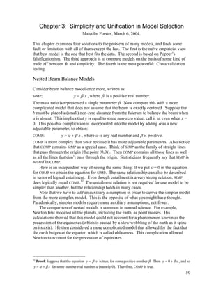
puzzling, especially with respect to the role Figure 3.1: A nine-degree polynomial fitted to
of simplicity. But as I will show in the
10 data points generated by the function y = x
penultimate section of this chapter, the
+ u, where u is a Gaussian error term of mean
0 and standard deviation ½.
same nuances arise in simpler comparisons
of nested models.
COMPTOO:
Why Naïve Empiricism is Wrong
Naïve empiricism is my name for the following solution to the problem of many models:
Choose the model that fits the data best, where the fit of the model is defined as the fit of
the best fitting member of the model. This proposal does not work because it favors the
most complex of the rival models under consideration, at least in the case of nested
models. The only exception is the rare case in which there may be a tie.
The proof is not only rigorous, but it is completely general because it doesn’t depend
on how fit is measured: Assume that SIMP is nested in COMP. Then the best fitting curve
in SIMP is also in COMP, and COMP will generally have even better fitting curves. And
since the special case in which they fit the data equally well almost never occurs, we can
conclude that more complex models invariably fit the data than simpler models nested in
them. More intuitively, complex models fit better because that are more flexible.
Complex families contain more curves and, therefore, have more ways of fitting the data.
This doesn’t prove that naïve empiricism is wrong in all model selection problems. It
merely shows that there seems to be problem when models are nested. It may not give
the wrong answer for all examples of comparing nested models. If there are only two
rival models, then the more complex model may be the right choice. For example,
observations of Halley’s comet show that it moves in an elliptical orbit. This hypothesis
is more complex than the hypothesis that Halley’s comet moves on a circle. But, even in
this example, naïve empiricism leads to absurd results if there is a hierarchy of nested
models of increasing complexity. Suppose we consider the hypothesis that the path is
circular with an added circular perturbation of a given radius and speed of rotation. Then
51

3. the circle is a special case of this more complex class of curves when the radius of the
added circle is zero; and so on, when circles on circles are added (this the construction
used by Copernicus and Ptolemy). There is a theorem of mathematics, called the
Fourier’s theorem, that says that an unbounded series of such perturbations can fit any
planetary trajectory (in a very broad class) to an arbitrary degree of accuracy. So, if there
are no constraints on what models are considered, naïve empiricism propels us up the
hierarchy until it finds a model that fits the data perfectly. But in doing so, we are fitting
the noise in the data at the expense of the signal behind the noise. This is the
phenomenon known as overfitting.
Similarly, it is well known that a n-degree polynomial (an equation of the form
y = β 0 + β1 x + β 2 x 2 + ! + β n x n ) can fit n +1 data points exactly. So, imagine that there
are 10 data points that are randomly scattered above and below a straight line. If our goal
were to predict new data, then it is generally agreed that it is not wise to use 10-degree
polynomial, especially for extrapolation beyond the range of the known data points (see
Fig. 3.1).
Complex models fit better, but we don’t want to move from a simple model to a more
complex model when it only fits better by some minute amount. The solution is to favor
SIMP unless there is a significant gain in fit in moving to COMP. This is exactly the idea
behind classical (Neyman-Pearson) hypothesis testing in statistics. Let α = 0 be the null
hypothesis and α ≠ 0 the alternative hypothesis. The Neyman-Pearson test is designed
to accept the simpler null hypothesis (SIMP) unless there is significant evidence against it.
There is widespread agreement amongst statisticians and scientists that some sort of trade
off between fit an simplicity is qualitatively correct. The problem with Neyman-Pearson
hypothesis testing is that the tradeoff is made according a merely conventional choice of
the “level of confidence”. There are two other methods, discussed later, that make the
tradeoff in a principled way. The trouble with them is that they do not take account of
indirect forms of confirmation.
Falsificationism as Model Selection
Popper’s methodology of falsificationism brings in the non-empirical virtue of
falsifiability, which Popper then equates with simplicity. The Popperian method proceeds
in two steps. Step 1: Discard all models that are falsified by the data. Step 2: From
amongst the surviving models, choose the model that is the most falsifiable. The second
step is motivated by the idea that new data may later falsify the favored model exactly
because it is the most vulnerable, but if it doesn’t, then the model has proved its worth.
From the previous section, it is clear that the fit of a
model with the data is a matter of degree. This means that
ELLIPSE
*
a Popperian must define what it means for a model to be
falsified by specifying some cutoff value such that any
CIRCLE
model that fits the data worse than this cutoff value counts
as falsified. While this introduces an element arbitrariness
into the model selection criterion, it is no worse than the
arbitrariness of the Neyman-Pearson cutoff.
The example that Popper discusses is actually an
Figure 3.2: CIRCLE is more
falsifiable than ELLIPSE.
example of model selection. Let CIRCLE be the hypothesis
that the planets move on a circle, while ELLIPSE is the
hypothesis that the planets move on an ellipse. CIRCLE is nested in ELLIPSE, so CIRCLE is
more falsifiable than ELLIPSE. A possible worlds diagram helps make the point (Fig.
52

4. 3.2). If the asterisk denotes the actual world, then its position on the diagram determines
the truth and falsity of all hypotheses. In the position shown, CIRCLE is false while
ELLIPSE is true. This is a world in which the planets orbit on non-circular ellipses. But
there is no possible world in which the opposite is true. It is impossible that CIRCLE is
true while ELLIPSE is false. Therefore, there are more possible worlds at which CIRCLE is
false, than possible worlds at which ELLIPSE is false. That is why CIRCLE is more
falsifiable than ELLIPSE. Notice that this has nothing to do with which world is the actual
world. Falsifiability is a non-empirical feature of models.
If the models are nested, the models are well ordered in terms of falsifiability, and in
such cases, it seems intuitively plausible to equate simplicity with falsifiability. But the
case of nested models is only one case. Popper wanted to equate simplicity with
falsifiability more generally—the problem is that it’s no longer clear how one compares
the falsifiability of non-nested models. His solution was to measure falsifiability in terms
of the number of data points needed to falsify the model. The comparison of SIMP and
COMP illustrates Popper’s idea. Any two data points will fit some line in COMP
perfectly.33 If that line does not pass through the origin, then the two points will falsify
every curve in SIMP. Therefore, SIMP is more falsifiable than COMP. SIMP is also simpler
than COMP. So, again, it seems that we can equate simplicity with falsifiability.
Notice that Popper’s definition of simplicity agrees with Priest’s conclusion that all
single curves are equally simple. For if we consider any single curve, then it is falsifiable
by a single data point.
We have two competing definitions of simplicity. The first is simplicity defined as
the fewness (paucity) of adjustable parameters and the second is Popper’s notion of
simplicity defined as falsifiability. It was Hempel (1966, p. 45) who saw that “the
desirable kind of simplification…achieved by a theory is not just a matter of increased
content; for if two unrelated hypotheses (e.g., Hooke’s law and Snell’s law) are
conjoined, the resulting conjunction tells us more, yet is not simpler, than either
component.”34 This is Hempel’s counterexample to Popper’s definition of simplicity.
The paucity of parameters definition of simplicity agrees with Hempel’s intuition. For
the conjunction of Hooke’s law and Snell’s laws has a greater number of adjustable
parameters than either law alone. The conjunction is more complex because the
conjuncts do not share parameters.
Another argument against Popper’s methodology has nothing to do with whether it
gives the right answer, but whether the rationale for the method makes sense. For
Popper, the goal of model selection is truth, assuming that one the rival models is true.
The problem is that all models, especially simple ones, are known to false from the
beginning—all models are idealizations. For example, the beam balance model assumes
that the beam is perfectly balanced, but it is not perfectly balanced; and it assumes that
the gravitational field strength is uniform, but it not perfectly uniform, and so on.
An immediate response is that the real goal is approximate truth, or closeness to the
truth. But if this response is taken seriously then it leads to a very different methodology.
Consider the sequence of nested models that are unfalsified. Without any loss of
generality, suppose that it is just SIMP and COMP. How is closeness to the truth to be
33
The only exception is when they both have the same x-coordinate. Then there is no function that fits the
data perfectly, because functions must assign a unique value of y to every value of x. And only those
curves that represent functions are allowed in curve fitting.
34
Hooke’s law says that the force exerted by a spring is proportional to the length that the spring in
stretched, where the constant of proportionality is called the stiffness of the spring, while Snell’s law says
the sine of the angle of the refraction of light is proportional to the sine of the angle of incidence, where the
constant of proportionality is the ratio of the refractive indices of the two transparent media at the interface.
53

5. defined? Presumably, it is defined in terms of the curve that best fits the true curve. But
now there is a problem. The fact that SIMP is nested in COMP implies that SIMP is never
closer to the truth than COMP. The proof is identical to the argument that showed that
SIMP never closer to the data than COMP—the only difference is that we are considering
fit to the truth rather than fit with data. Again, the argument does not depend on how
closeness to the truth is defined: Suppose C* is the hypothesis in SIMP that is the closest
to the truth. Then C* is also in COMP, so the closest member of COMP to the truth is either
C*, or something that is even closer to the truth, which completes the proof.
Popper’s methodology, or any methodology that aims to select a model that is closest
to the truth, should choose the most complex of the unfalsified models. In fact, it can
even skip step 1 and immediately choose the most complex model, the most complex
model in a nested hierarchy of models is always the closer to the truth than any simpler
model (or equally close).
One response is to say the aim is not to choose the model that is closest to the truth,
but to choose a curve that is closest to the truth. This is an important distinction. The
goal now makes sense, but Popper’s methodology does not achieve this goal. The
procedure is to take the curve that best fits the data from each model, and compare them.
Step 1 eliminates curves that are falsified by the data. So far, so good. But now step 2
says that we should favor the curve that is simplest. But according to Popper’s definition
of simplicity, all curves are equally simple. Popper’s methodology does not make sense
as a method of curve selection.
I suspect that Popperians will reject the premise that the closeness of a model to the
truth is defined purely in terms of the predictive accuracy of the curves it contains. It
should also depend on how well the theoretical ontology assumed by the model
corresponds to the reality. But it should be clear from this discussion that it is hard to
support these realist intuitions if one is limited to the methodology of falsificationism. In
particular, there is nothing in the Popperian toolbox that takes account of indirect
confirmation.
Goodness-of-Fit and its Bias
It is time to see how fit is standardly defined, so that we can better understand how the
problem with naïve empiricism might be fixed. Consider some particular model, viewed
as a family of curves. For example, SIMP is the family of straight lines that pass through
the origin (Fig. 3.3). Each curve (lines in this case) in the family has a specific slope
which is equal to the mass ratio m(a)/m(b), now labeled β.
When curve fitting is mediated by
y
models, there is no longer any guarantee
R1
that there is a curve in the family that fits
the data perfectly. This immediately
4
raises the question: If no curve fits
R
perfectly, how do we define the best
Datum 3
fitting curve? This question has a famous
2
answer in terms of the method of least
Datum 2
squares.
Datum 1
Consider the data points in Fig. 3.3
and an arbitrary line in SIMP, such as the
x
1
2
3
one labeled R 1 . What is the ‘distance’ of
this curve from the data? A standard
Figure 3.3: R fits the data better than R1.
54

6. answer is the sum of squared residues (SSR), where the residues are defined as the ydistances between the curve and the data points. The residues are the lengths of the
vertical lines drawn in Fig. 3.3. If the vertical line is below the curve, then the residue is
negative. The SSR is always greater than or equal to zero, and equal to zero if and only if
the curve passes through all the data points exactly. Thus, the SSR is an intuitively good
measure of the discrepancy between a curve and the data.
Now define the curve that best fits the data as the curve that has the least SSR. Recall
that there is a one-to-one correspondence between numerical values assigned to the
parameters of a model and the curves in the model. Any assignment of numbers to all the
adjustable parameters determines a unique curve, and vice versa: Any given curve has a
unique set of parameter values. So, in particular, the best fitting curve automatically
assigns numerical values to all the adjustable parameters. These values are called the
estimated values of the parameters. When fit is defined in terms of the SSR, the method
of parameter estimation is “the method of least squares”.
The process of fitting a model to the data yields a unique best fitting curve.35 The
values of the parameters determined by this curve are often denoted by a hat. Thus, the
ˆ
curve in SIMP that best fits the seen data is denoted by y = β x . This curve makes precise
predictions, whereas the model does not.
However, the problem is now more complicated. We need a solution to the problem
of many models, and we already know that naïve empiricism does not work. To fix the
problem, we need to analyze where the procedure goes wrong.
The goodness-of-fit score for each model is calculated in the following way:
Step 1: Determine the curve that best fits the data. Denote this curve by C.
Step 2: Consider a single datum. Record the residue between this datum and the curve C
and square this value.
Step 3: Repeat this procedure for all N data.
Step 4: Average the scores. The result is the SSR of C, divided by N.
The resulting score actually measures the badness-of-fit between the model and the data.
The cognate notion of goodness-of-fit could be defined as minus this score, but this
complication can be safely ignored for our purposes.
The reason that we take the average SSR in step 4 is that we want to use the
goodness-of-fit score to estimate how well the model will predict a “typical” data point.
The goal is the same as the goal of simple enumerative induction—to judge how well the
“induced” hypothesis predicts the next instance.
The problem is that each datum has been used twice. It is first used in the
construction of the “induced” hypothesis, for the curve that “represents” a model is the
one that best fits all the data. So, when the same data are used to estimate the predictive
error of a typical datum of the same kind, there is a bias in the estimate. The estimated
error is smaller than it should be because the curve has been “constructed” in order to
minimize these errors. The flexibility of complex models makes them especially good at
doing this. This is the reason for the phenomenon of overfitting (Fig. 3.1).
Nevertheless, if a particular model is chosen by a model selection method, then this is
the curve that we will use for prediction. So, the only correctable problem arises from the
use the goodness-of-fit scores in comparing the models. If the scores were too low by an
equal amount for each model, then the bias would not matter. But this is not true, for
complex models have a greater tendency to overfit the data.
35
There are exceptions to this, for example when the model contains more adjustable parameters than there
are data. Scientists tend avoid such models.
55

7. While this is the cause of the problem, it may also be the solution. For there is some
hope that the degree of overfitting may be related to complexity in a very simple way. If
we knew that, then it might be possible to correct the goodness-of-fit score in principled
way. There is a surprisingly general theorem in the mathematical statistics (Akaike 1973)
that fulfills this hope. It is not my purpose to delve into the details of this theorem (see
Forster and Sober 1994 for an introduction). Nor is there any need to defend the Akaike
model selection criterion (AIC) against the host of alternative methods. In fact, my
purpose is to point out that they all have very similar limitations.
Akaike’s theorem leads to the following conclusion: The overfitting bias in the
goodness-of-fit score can be corrected by a multiplicative factor equal to
( N + k ) ( N − k ) , where k is the number of adjustable parameters in the model. That is,
the following quantity is an approximately unbiased estimate of the expected predictive
error of a model:
SSR N + k
,
N N −k
Terms of order (k N )3 have been dropped. The proof of this formula in a coin tossing
example is found in a later chapter, along with an independent derivation of it from
Akaike’s theorem.
When models are compared according to this corrected score, it also implements the
Neyman-Pearson idea that the simpler model is selected if there is no significantly
greater fit achieve by the more complex model. The difference is that the definition of
what counts as “significantly greater” is determined in a principled way. The
introduction of simplicity into the formula does not assume that nature is always simple.
Complex models do and should often win. Rather, the simplicity of the model is used to
correct the overfitting error caused by the model.
It is very clear in the Akaike framework that the penalty for complexity is only
designed to correct for overfitting. Moreover, the size of the penalty needed to correct
overfitting decreases as the number of data increases (assuming that the number of
adjustable parameters is fixed). In the limit, ( N + k ) ( N − k ) is equal to 1. Perhaps the
most intuitive way of seeing why this should be so is in terms of the signal and noise
metaphor. When the number of data is large, the randomness of the noise allows the
trend, or regularity, in the data (the signal) to be clearly seen.
Of course, if one insists on climbing up the hierarchy of nested models to models that
have almost as many parameters as data points, then the correction factor is still
important. But this is not common practice, and it is not the case in any of the examples
here. The point is that the Akaike model selection criterion makes the same choice as
naïve empiricism in this special case. This is a problem because goodness-of-fit ignores
indirect confirmation, which do not disappear in the large data limit.
Leave-One-Out Cross Validation
There is a more direct way of comparing models that has the advantage of avoiding the
problem of overfitting at the beginning—there is no problem, so there is no need to use
simplicity to correct the problem. Recall that overfitting arises from the fact that the data
are used twice—once in “constructing” the best fitting curve, and then in goodness-of-fit
score for the model. There is a simple way of avoiding this double-usage of the data,
which is known as leave-one-out cross validation (CV). The CV score is calculated for
each model in the following way.
56

8. Step 1: Choose one data point, and find the curve that best fits the remaining N−1 data
points.
Step 2: Record the residue between the y-value given by the curve determined in step 1
and the observed value of y for this datum Then square the residue so that we
have a non-negative number.
Step 3: Repeat this procedure for all N data.
Step 4: Sum the scores and divide by N.
The key point is the left out datum is not used to “construct” the curve in step 1. The
discrepancy score is a straightforward estimate of how good the model is at prediction—
it is not a measure of how well the model is able to accommodate the datum. This is an
important distinction, because complex models have the notoriously bad habit of
accommodating data very well. On the other hand, complex models are better at
providing more curves that are closer to the true curve. By avoiding the overfitting bias,
the comparison of CV scores places all models on an even playing field, where the data
becomes a fair arbiter.
Just in case anyone is not convinced that the difference between the goodness of fit
score and the CV score is real, here is a proof that not only is the CV score always greater
in total, but it is also greater for each datum. Without loss of generality, consider datum
1. Label the curve best fits to the total data as C, and the curve that best fits the N−1 data
as C1 . Let E be the squared residue of datum 1 relative to C, and let E1 be the squared
residue of datum 1 relative to C1 . What we aim to prove is that E1 ≥ E . Let F be sum
of the SSR of the remaining data relative to C , while F1 is the SSR of the remaining data
relative to C1 . Both F and F1 are the sum of N −1 squared residues. By definition, C fits
the total data at least as well as C1 . Moreover, the SSR for C relative to the total data is
just E + F while the SSR of C1 relative to the total data is E1 + F1 . Therefore,
E1 + F1 ≥ E + F . On the other hand, C1 fits the N − 1 data at least as well as C, again by
definition of “best fitting”. Therefore, F ≥ F1 . This implies that E + F ≥ E + F1 . Putting
the two inequalities together: E1 + F1 ≥ E + F ≥ E + F1 , which implies
that E1 + F1 ≥ E + F1 . That is, E1 ≥ E , which is what we set out to prove.
It is clear that models compared in terms of their CV scores are being compared in
terms of their estimated predictive accuracy, as distinct from their ability to merely
accommodate data. The idea is very simple. The predictive success of the model within
the seen data is used to estimate its success in predicting new data (of the same kind) It is
based on a simple inductive inference: Past predictive success is the best indicator of
future predictive success.
There is a theorem proved by Stone (1977) that shows that leave-one-out CV score is
asymptotically equal to the Akaike score for large N. This shows that both have the same
goal—to estimate how good the model is at prediction. A rigorous analysis in a later
chapter will show that the equivalence holds in a coin tossing example even for small N.
Note that it is very clear that leave-one-out CV comparisons work equally for nested
or non-nested models. The only requirement is that they are compared against the same
set of data. The same is true of Akaike’s method.
For large N both methods reduce to the method of naïve empiricism (in the
comparison of relatively simple models). This is clear in the case of leave-one-out CV
because the curves that best fit N −1 data points will be imperceptibly close the curve that
best fits all data points.
57

9. The goals are the same. But the goal of leave-one-out CV is not to judge the
predictive accuracy of any prediction. It is clearly a measure of how well the model is
able to predict a randomly selected data point of the same kind as the seen data. The goal
of Akaike’s method is also the prediction of data of the same kind.
One might ask: How it could be otherwise? How could the seen data be used to judge
the accuracy of predictions of a different kind? This is where indirect confirmation plays
a very important role. Indirect confirmation is a kind of cross validation test, albeit one
very different from leave-one-out CV. This point is most obvious in the case of unified
models.
Confirmation of Unified Models
When the beam balance model is derived from Newton’s theory, mass ratios appear as
coefficients in the equation. When we apply the model to a single pair of objects
repeated hung at different places on the beam, it makes no empirical difference if the
coefficient is viewed as some meaningless adjustable parameter β. But does it ever make
an empirical difference? The answer is ‘yes’ because different mass ratios are related to
each other by mathematical identities. These identities are lost if the mass ratios are
replaced by a sequence of unconnected β coefficients.
With respect to a single application of the beam balance model applied to a single
pair of objects {a, b}, the following equations are equivalent because they define the
same set of curves:
m( a )
x , and y = β x .
m(b)
But, when we extend the model, for example, to apply to three pairs of objects, {a, b},
{b, c}, and {a, c}, then the situation is different. The three pairs are used in three beam
balance experiments. There are three equations in the model, one for each of the three
experiments.
y=
UNIFIED:
y1 =
m( a )
m(b)
m( a )
x1 , y2 =
x2 , and y3 =
x3 .
m(b)
m(c )
m(c )
In contrast, define COMP by the equations:
COMP:
y1 = α x1 , y2 = β x2 , and y3 = γ x3 .
While COMP may look simpler than UNIFIED, it is not according to our definition of
simplicity. The adjustable parameters of UNIFIED are m(a) , m(b) , and m(c) , while
those of COMP are α , β , and γ . At first, one might conclude that the models have the
same number of adjustable parameters. However, there is a way of counting adjustable
parameters such that UNIFIED has fewer adjustable parameters, and hence is simpler.
This is because the third mass ratio, m(a ) m(c) is equal to the product of the other two
mass ratios according to the mathematical constraint:
m(a) m(a ) m(b)
=
.
m(c) m(b) m(c)
Note that what I am calling a constraint (in reverence to Sneed 1971) is not something
added to the model. It is a part of the model.
A second way of comparing the simplicity of the models is to assign one mass the
role of being the unit mass. Set m(c) = 1 . Then UNIFIED is written as:
CONSTRAINT:
58

10. m( a )
x1 , y2 = m(b) x2 , and y3 = m(a) x3 .
m(b)
Again, the number of adjustable parameters is 2, not 3.
Another way of making the same point is to rewrite the unified model as:
UNIFIED:
UNIFIED:
y1 =
y1 = α x1 , y2 = β x2 , and y3 = αβ x3 .
Again, we see that UNIFIED has only two independently adjustable parameters. It is also
clear that UNIFIED is nested in COMP because UNIFIED is a special case of COMP with the
added constraint that γ = αβ . The earlier proof that simpler models never fit the data
better than more complex models extends straightforwardly to these two models.
The only complication is that these models are not families of curves, but families of
curve triples. For example, COMP is the family of all curve triples (C1 , C2 , C3 ) , where for
example C1 is a curve described by the equation y1 = 2 x1 , C2 is a curve described by the
equation y2 = 3x2 , and C3 is a curve described by the equation y3 = 4 x3 . Since each
curve is uniquely defined by its slope, we could alternatively represent COMP as the
family of all triples of numbers (α , β , γ ) . These include triples of the form (α , β , αβ ) as
special cases. Therefore, all the curve triples in UNIFIED are contained in COMP, and any
fit that UNIFIED achieves can be equaled or exceeded by COMP. This applies to any kind
of fit. It applies to fit with the true curve (more precisely, the triple of true curves), as
well as fit with data.
No matter how one looks at it, UNIFIED is simpler than COMP. Unification is
therefore a species of simplicity. Yet it is also clear that unification is not merely a
species of simplicity. Unification, as the name implies, has a conceptual dimension. In
particular, define “a is more massive than b” to mean that m(a ) m(b) > 1 . Now the
CONSTRAINT implies that the following argument is deductively valid:
a is more massive than b
b is more massive than c

a is more massive than c
For it is mathematically impossible that m(a ) m(b) > 1 , m(b) m(c) > 1 , and
m(a ) m(c) ≤ 1 . In contrast to this, let the made-up predicate “massier than” define the
COMP mass relation, where by definition, “a is massier than b” if and only if α > 1. Then
the corresponding argument is not deductively valid:
a is massier than b
b is massier than c

a is massier than c
That is, the mass relation in the UNIFIED representation is a transitive relation, while the
COMP concept is not. The unified concept of mass is logically stronger.
Just as before, there are two conceivable ways of dealing with the overfitting bias
inherent in the more complex model. The Akaike strategy is to add a penalty for
complexity. However, it is not clear that this criterion will perform well in this example.
The first reason is that, according to at least one analysis in the literature (Kieseppä
1997), Akaike’s theorem has trouble applying to functions that are nonlinear in the
parameters, as is the case in y3 = αβ x3 . It would be interesting to verify this claim using
computer simulations, but I have not done so at the present time.
59

11. In any case, leave-one-out CV scores still do what they are supposed to do. And it is
still clear that both methods will reduce to naïve empiricism in the large number limit.
That is all that is required in the following argument.
Any method of model selection that reduces to naïve empiricism in the large data
limit will fail to distinguish between UNIFIED and COMP when the data are sufficiently
numerous and varied (covering all three experiments).36 The reason is that all model
selection criteria that merely compensate for overfitting reduce to naïve empiricism
(assuming that the models are relatively simple, which is true in this example). More
precisely, assume that the constraint γ = αβ is true, so that the data conform to this
constraint. This regularity in data does not lend any support to unified model if the
models are compared in terms of goodness-of-fit with the total evidence. Leave-one-out
cross validation will do no better, because it is also equivalent to naïve empiricism in the
large data limit.
At the same time, two things seem clear: (1) When the models are extended to a
larger set of objects, then the transitivity property of the unified (Newtonian)
representation provides the extended model with greater predictive power. In contrast,
COMP imposes no relations amongst data when it is extended in the same way. (2) There
does exist empirical evidence in favor of the unified model. For all three mass ratios are
independently measured by the data—once measured directly by the data in the
experiment in which the equation applies, and independently via the intra-model
CONSTRAINT. The agreement of these independent measurements is a kind of
generalized cross validation test, which provides empirical support for the unified model
that the disunified model does not have. COMP is not able to measure its parameters
indirectly, so there is no indirect confirmation involved. The sum of the evidence for
COMP is nothing more than the sum of its evidence within the three experiments.
In the large data limit, UNIFIED and COMP do equally well according to the leave-oneout CV score and the Akaike criterion, and according to any criterion that adds a penalty
for complexity that is merely designed to correct for overfitting. Yet UNIFIED is a better
model than COMP, and there exists empirical evidence that supports that conclusion.
Does this mean that the standard model selection criteria fail to do what they are designed
to do? Here we must be careful to evaluate model selection methods with respect a
specific goal.
The judgments of leave-one-out cross validation and the Akaike criterion are
absolutely correct relative to the goal of selecting a model that is good at predicting data
of the same kind. There is no argument against the effectiveness of these model selection
criteria in achieving this goal. The example merely highlights the fact already noted—
that the goal of Akaike’s method and leave-one-out CV is limited to the prediction of
data of the same kind. The point is that cross validation tests in general are not limited in
the same way.
The agreement of independent measurements of the mass ratios provides empirical
support for the existence of Newtonian masses, including the transitivity the “more
massive than” relation. This, in turn, provides some evidence for accuracy of predictions
of the extended model in beam balance experiments with different pairs of objects.
36
I first learned the argument from Busemeyer and Wang (2000), and verified it using computer
simulations in Forster (2000). The argument is sketched in Forster (2002). The present version of the
argument is more convincing, I think, because it does not rely on computer simulations, and the
consequences of the argument are clearer.
60

12. To make the point more concretely, consider the experiment in which all three
objects, a, b and c are hung together on the beam (Fig. 3.4). By using the same auxiliary
assumptions as before, the Newtonian model derived for this experiment is:
NEWTON:
y=
m( a )
m (c )
x+
z.
m(b)
m(b)
In terms of the α and β parameters, this is:
NEWTON:
y =αx+ z β .
If COMP extends to this situation at
x
y
all, it will do so by using the
z
equation y = δ x + ε z . The
Newtonian theory not only has a
c
a
b
principled way of determining the
form of the equation, but it also
reuses the same theoretical quantities
as before, whose values have been
Figure 3.4: A beam balance with three masses.
measured in the first three
experiments.
At end the of the previous section, I asked how data of one kind could possibly
support predictions of a different kind. The answer is surprisingly Kuhnian. The duckrabbit metaphor invites the idea that new theories impose relations on the data. For
Kuhn, this is a purely subjectively feature of theories that causes a breakdown in
communication. For me, the novel predictions are entailed by structural features of the
theory that can be empirically confirmed—the transitivity of relation “more massive
than” is just one example. The empirical support for lateral predictions of this kind is not
taken into account by the goodness-of-fit score, even when it is corrected for overfitting.
The support for “lateral” predictions is indirect. The evidence (that is, the agreement
of independent measurements) supports the mass ratio representation, and its logical
properties, which supports predictions in other applications.
There is a sense in which the inference is straightforwardly inductivist in nature. At
the same time, it is not a simple kind of inductivist inference, for it depends crucially on
the introduction of theoretical quantities, and on their logical properties. Conceptual
innovation is also allowed by inference to the best explanation. The difference is that the
present account does not rely on any vague notion of “explanation” or on any unspecified
account of what is best. This is why curve fitting, properly understood, succeeds in
finding middle ground between two philosophical doctrines, one being “trivial” and other
being “false”.
If the inference is viewed as inductive, then its justification depends on an assumption
about the uniformity of nature. But the premise is not the unqualified premise that nature
is uniform in all respects. The premise is that nature is uniform with respect to the
logical properties of mass ratios. Any mention of “induction” invites the standard
skeptical response to the effect that it is always logically possible that the uniformity
premise is false. In my view, this reaction is based on a misunderstanding of the
problem. The problem is not to provide a theory of confirmation that works in all
possible worlds. There is not such thing.
The first part of the problem is to see how confirmation works in the quantitative
sciences, to the extent that it does work, and to understand why it works in the actual
world. My answer is “curve fitting, properly understood”. The first part of the solution to
61

13. describe inductive inferences actually used in science. The second question is to ask
what the world must be like in order that inductive inferences used in science work as
well as they do. The solution is that the world is uniform in some respects. This part of
the answer is formulated within the vocabulary of the scientific theory under
consideration. But the answer is not viciously circular—for the circle is broken by the
empirical support for the uniformity.
At the same time, scientists entrenched in new theory may overlook the fact the new
theoretical structure has empirical support. Ask any Newtonian why it is possible to
predict m(a ) m(c) from m(a ) m(b) and m(b) m(c) . After a little thought, they will
refer you to the CONSTRAINT. If you then ask why they believe in this identity, they will
assume that you are mathematically challenged, and provide a simple algebraic proof. It
is hardly surprising that this answer is unconvincing to pre-Newtonians. What preNewtonians want to know is: Why use the mass ratio representation in the first place? A
typical answer to this question is likely to be “because the theory says so, and the theory
is supported by the evidence”. The problem is that standard views about the nature of
evidence, especially amongst statisticians and philosophers, do not justify this response.
In sum, there is good news and bad news for empiricism. The bad news is that
goodness-of-fit is not good enough, nor corrected goodness-of-fit, nor leave-one-out
cross validation. The good news is that there is a more general ways of understanding
what evidential fit means that includes indirection confirmation, general cross validation,
and the agreement of independent measurements.
What role does simplicity play in this more advanced version of empiricism? It is
clear that no cross validation depend explicitly on any notion of simplicity. But is it a
merely accidental that a simpler model succeeds where a more complex model fails? It is
intuitively clear that unification, viewed as a species of simplicity, did play a role in the
indirect confirmation of the unified model. For it is the necessary connection between
different parts of the model that leads to the extra predictive power, and this is traced
back to the fewer number of independently adjustable parameters. Simplicity is playing a
dual role.
First, simplicity plays a role in minimizing overfitting errors. Complex models are
not avoided because of any intrinsic disadvantage with respect to their potential to make
accurate predictions of the same kind as the seen data. This is very clear in the case of
nested models, for any predictively accurate curve contained in the simpler is also
contained in the more complex model. In the large data limit, this curve is successfully
picked out, which is why both models are equally good at predicting the “next instance”.
When the data size is intermediate, it is important to understand that the leave-one-out
CV score only corrects the bias in the goodness-of-fit score. It does not correct the
overfitting error in the curve that is finally used to make predictions. So, one reason why
simpler models tend to be favored is that their best fitting curves may be closer to the true
curve than the best fitting curve in the complex model. In fact, simpler models can be
favored for this reason even when they are false (they do not contain the “true” curve)
even when the complex model is true. Part of the goal of the comparison is pick the best
curve estimated from the data at hand, rather than model that is (potentially) best model
at predicting data of the same kind.
In its second role, the simplicity of a model is important because it introduces intramodel constraints that produce internal predictions. If these predictions are confirmed—
that is, if the independent measurements of parameters agree—then this produces a kind
of fit between the model and its evidence that is not taken into account by a model
selection method designed to correct, or avoid, overfitting bias. The simpler model has a
62

14. kind of advantage that has nothing to do with how close any of its curves are to the true
curve. In fact the closeness of these curves to the true curve provides no information
about the predictive accuracy of curves in an extended model, as is clearly demonstrated
in the case of COMP.
Even for unified models, it may not clear how the model should be extended. For
example, imagine that scientists are unaware that mass ratios measured in beam balance
experiments can predict the amount that the same objects stretch a spring (Hooke’s law).
Suppose that the “beam balance masses” of objects d, e, and f are measured in an
experiment. Then it is discovered empirically that d, e, and f stretch a spring by an
amount proportional to the “beam balance mass” of these objects. This supports the
conjecture that spring masses are identical to beam balance masses, and the
representational properties of beam balance mass automatically extends to spring masses.
Because the extension of models may be open-ended in this way, it is natural to view the
agreement of independent measurements as a verification not of any specific kind of
predictive accuracy, but as a verification that these quantities really exist. For that
reason, the agreement of independent measurements is viewed most naturally as
confirmation that Newtonian masses really exist. The evidence is most naturally viewed
as supporting a realist interpretation of the model.
Define COMP+ to be COMP combined with the added constraint that γ = αβ . Is there
any principled difference between this model and the UNIFIED model? At first sight,
these models appear to be empirically equivalent. Indeed they are empirically equivalent
with respect to the seen data in the three experiments and with respect to any new data of
the same kind. At this point, it tempting to appeal to explanation once more: UNIFIED
explains the seen data better COMP+ because the empirical regularity, γ = αβ , is explained
as a mathematical identity. I have no objection to this idea except to say that it does little
more than name an intuition. I would rather point out that added constraint COMP+ is
restricted to these three experiment. It does not impose any constraints on disparate
phenomena. It produces no predictive power.
One might object that UNIFIED should also be understood in this restricted way. But
this would be to ignore the role of the background theory. The theory and its formalism
provides the predictive power. COMP+ is not embedded in a theory, and therefore makes
no automatic connections with disparate. For indirect confirmation to succeed, one must
take the first step, which is to introduce a mathematical formalism that makes
connections between disparate phenomena in an automatic way.
Newtonian mechanics does this in a way that COMP+ does not. The predictions can
then be tested, and if the predictions are right, then the formalism, or aspects of the
formalism, is empirically confirmed. If it’s disconfirmed, then a new formalism takes its
place. Gerrymandered models such as COMP+ can provide stop-gap solutions, but they are
eventually replaced by a form of representation that does the job automatically for that is
what drives the whole process forward. This is the point at which Popper’s intuitions
about the value of falsifiability seem right to me. It is also a point at which the
deducibility of predictions becomes important.
All of this is intuitively clear in the beam balance example. But does it apply to other
examples? The next section shows how an empiricist can argue that Copernican
astronomy was better supported than Ptolemaic astronomy by the known observations at
its inception. The argument is not based on the claim that Copernicus’s theory was better
at predicting “the next instance”. It may have been that the church hoped that
Copernicus’s theory would be better than Ptolemy’s at predicting the dates for Easter
each year, but there seems to be a consensus amongst historians that it was not more
63

15. successful in this way. But the predictive equivalence of Copernican and Ptolemaic
astronomy in this sense amounts to nothing more an equivalence in leave-one-out CV
scores. As the beam balance example shows clearly, leave-one-out CV scores do not
exhaust the total empirical evidence. Copernicus could have argued for his theory on
other grounds. Indeed, Copernicus argued for his theory by pointing indirect forms of
confirmation. He also appealed to simplicity, which has puzzled commentators over the
centuries.
The Harmony of the Heavens
The idea that simplicity, or parsimony, is important in science pre-dated Copernicus
(1473 - 1543) by 200 years. The law of parsimony, or Ockham’s razor (also spelt
‘Occam’), is named after William of Ockham (1285 - 1347/49). He stated that “entities
are not to be multiplied beyond necessity”. The problem with Ockham’s “law” is that it
is notoriously vague. What counts as an entity? For what purpose are entities necessary?
When are entities postulated beyond necessity? Most importantly, why should parsimony
be a mark of good science?
Copernicus argued that his heliocentric theory of planetary motion endowed one cause
(the motion of the earth around the sun) with many effects (the apparent motions of the
planets), while his predecessor (Ptolemy) unwittingly duplicated the earth’s motion many
times in order to “explain” the same effects. Perhaps Copernicus was initially struck by
the fact that there was a circle in each of Ptolemy’s planetary models whose period of
revolution was (approximately) one year—viz. the time it takes the earth to circle the sun.
His mathematical demonstration that the earth’s motion could be viewed as an
component of the motion of every planet did prove that the earth’s motion around the sun
could be seen as the common “cause” of each of these separate “effects”. In Copernicus’s
own words:
We thus follow Nature, who producing nothing in vain or superfluous often prefers to
endow one cause with many effects. Though these views are difficult, contrary to
expectation, and certainly unusual, yet in the sequel we shall, God willing, make them
abundantly clear at least to the mathematicians.37
Copernicus tells us why parsimony is the mark of true science: Nature “prefers to endow
one cause with many effects”. His idea that the nature of reality behind the phenomena is
simpler than the phenomena itself has been sharply criticized by philosophers over the
ages, and correctly so. There are many counterexamples. Consider that case of
thermodynamics, in which quite simple phenomenological regularities, such as Boyle’s
law, arise from a highly complex array of intermolecular interactions.
Newton’s version of Ockham’s razor appeared in the Principia at the beginning of his
rules of philosophizing: Rule 1: “We are to admit no more causes of natural things than
such as are both true and sufficient to explain their appearances”. In the sentence
following this, Newton makes the same Copernican appeal to the simplicity of Nature:
“To this purpose the philosophers say that Nature does nothing in vain, and more is in
vain when less will serve; for Nature is pleased with simplicity, and affects not the pomp
of superfluous causes.”
It is hardly surprising that so many historians and philosophers have found such
appeals to simplicity of Nature puzzling. In his influential book on the Copernican
37
De Revolutionibus, Book I, Chapter 10.
64

16. revolution (from Copernicus to Newton), Kuhn (1957, p.181) claims that the “harmony”
of Copernicus’ system appeals to an “aesthetic sense, and that alone”:
The sum of evidence drawn from harmony is nothing if not impressive. But it
may well be nothing. “Harmony” seems a strange basis on which to argue for
the Earth’s motion, particularly since the harmony is so obscured by the
complex multitude of circles that make up the full Copernican system.
Copernicus’ arguments are not pragmatic. They appeal, if at all, not to the
utilitarian sense of the practicing astronomer but to his aesthetic sense and to
that alone.
In my view, there is a sense in which the evidence is drawn from Harmony. For the
evidence that Copernicus points to arises from cross validation predictions that owe their
existence to the greater unification of his system. But this unification is useless as an
argument for the theory if these predictions are not borne out by the observational data.
This is the point that is not properly appreciated.
My analysis is not presented as an exegesis of
Mars
Copernicus, or any other thinker. To the contrary, I have
already argued that the relevance of simplicity was
misunderstood by Copernicus and Newton themselves.
Earth
It was well known to the ancients that planets, such as
Mars, follow the same line of stars traversed by the sun (the
constellations known as the signs of the zodiac). Yet
occasionally, the planets outside the earth’s orbit would slow
Sun
down and reverse their direction of motion, and then turn
around and continue in their usual direction of motion. This
Figure 3.5: Copernicus’s
backwards motion is called retrograde motion.
theory implies that Mars’
retrograde motion occurs
The phenomenon is easiest to explain in terms of the
only when the sun and the
basic Copernican model. The earth’s orbit is inside Mars’s
planet are on opposite
orbit, but inner planets circle the sun more frequently than
sides of the earth.
outer planets. So, periodically, the earth will overtake Mars
in its orbit. When it does, it’s like being in a car traveling at 60 kilometers per hour that
is overtaking another car traveling at 30 kilometers per hour. Both cars are moving
forward, but the slower car appears to be moving backwards from the point of view of the
faster moving vehicle.
But, stranger than that, imagine that whenever the moon is in the night sky near Mars,
then the moon is fully illuminated by the sun if and only if Mars is in retrograde motion.
This is a striking phenomenon, for it might appear that the moon and the sun have some
strange power over the planet Mars. The phenomenon is easy to understand on the
Copernican theory (Fig. 3.5). For it is obvious that the earth can only overtake Mars
when they are on the same side of the sun.
It is important to understand that the evidence that Copernicus’s highlighted was not
merely that the outer planets move backwards from time to time, but that this retrograde
motion occurs if and only if the sun, earth, and Mars are lined up in that order. In the
language of astronomy, the phenomenon was that the retrograde motion of the outer
planets always occurs in opposition to the sun.
Ptolemy’s theory was unable to predict this phenomenon. But, contrary to what
Popper’s methodology might suggest, it was not falsified by it either. For Ptolemy’s
65

17. theory was able to accommodate the phenomenon perfectly well. The distinction
between prediction and accommodation is crucial.38
The first thing to understand is how Ptolemy could account for retrograde motion at
all. In his model of planetary motion, the orbits of each planet were unconnected to each
other.39 Ptolemy’s planetary model consisted of unconnected parts (just like COMP in the
previous section). Having Mars circling on a single circle centered near the earth cannot
account for retrograde motion. So, Ptolemy needed a second circle, called an epicycle,
whose center rotated on the circumference of the main circle, called the deferent (Fig.
3.6).
There is no problem arising from the fact Ptolemy
needed two circles to account retrograde motion. For
Mars
Copernicus uses two circles as well, one for the earth and
one for the planet. The problem is that Ptolemy has to
account for the correlation between the occurrence of
retrograde motion and the position of the sun by making
Earth
sure that the sun is in the right place. He can only do this
by making sure that the time it takes Mars to revolve on its
epicycle is the same time it takes for the sun to move
around the earth—namely, one year. Therefore, Ptolemy
Figure 3.6: Ptolemy’s basic
ended up duplicating the motion of the earth in Mars’s
model of the retrograde
epicycle, and similarly for all the outer planets.
motion of Mars. See text for
details.
Copernicus does not duplicate the earth’s motion to
account for each planet. His theory is more unified. This
is what Copernicus is referring to when he says: “We thus follow Nature, who producing
nothing in vain or superfluous often prefers to endow one cause with many effects.”
Now we can see why Ptolemy had no problem accommodating the phenomenon.
The equality of the period motion of the main epicycles on the outer planets is merely a
coincidence in Ptolemy’s view. It is not entailed by his theory, nor by any of his models.
But it is correctly entailed by his fitted model (just as the regularity γ = αβ is entailed by
COMP after it is fitted to data). That is why Ptolemy’s theory is not falsified by the
phenomenon.
In Copernicus’s theory, the equality of the periods of the motion of these many circles
in Ptolemy’s model becomes a mathematical necessity because all of the circles are
replaced by one circle—the circle on which the earth orbits the sun. It is this reduction in
the number of circles (accompanied by a reduction in the number of adjustable
parameters) that makes Copernicus’s theory more harmonious, or simpler, or more
unified. For this is what explains the added predictive power of the Copernican models.
Naturally, the fundamental argument in favor of Copernicus’s theory requires that this
predictive power is translated into predictive success, and there was certainly sufficient
data available in Copernicus’s time to show that the prediction was correct.
38
Unfortunately, many philosophers of science, such as White (2003), have characterized the distinction in
psychological or historical terms. But it is clear in this example that prediction is of facts that were well
known prior to Copernicus. There is no “prediction in advance”. The distinction between prediction and
accommodation is a logical distinction. See the section in chapter 1 on historical versus logical theories of
confirmation.
39
In a manuscript lost to the Western world for many centuries, but preserved by Persian astronomers,
Ptolemy did place the planets in an order—in fact, the correct order. But his planetary hypothesis still
duplicated the motion of the earth for each planet, or in Copernicus’s words, Ptolemy failed to endow many
effects with one cause.
66

18. Historians of science, like Kuhn, have been perplexed by Copernicus’s appeal to
harmony. They point to the fact that Copernicus’s final model also added epicycles to his
circles, and epicycles on epicycles, just as Ptolemy did. In fact, they eagerly point out
that the total number of circles in Copernicus’s final model exceeded the total number of
circles used by Ptolemy. This confusion arises from their failure to distinguish between
the two roles of simplicity. The fact that Copernicus theory is unified in the way
described is all that is needed to explain the extra predictive power of the theory. The
total simplicity of any particular model does not matter.
The fact that Copernicus used more circles in total might be explained by the fact that
he had a larger set of data available to him. In hindsight, we know that he would need an
infinite number of epicycles to replicate Keplerian motion, and so a greater number of
data points would propel any circle on circle construction to increasing levels of
complexity. The same fact would explain why his theory was not great at “predicting the
next instance”. For if every new cluster of data points drives the theory towards a more
complex model in order to maximize the leave-one-out CV score, then it is because the
previously best fitting model did not predict the new cluster of data very well.
If this analysis is correct, then it has an extremely important epistemological
consequence. It means that the indirect confirmation for a model can still work even
when a model is relatively poor at predicting data “of the same kind”. That is, a model
does not have to be accurate in order to benefit from this very important from of
confirmation. Moreover, many models of theory can receive this support, so that the
evidence can be viewed as supporting the structural features that these models have in
common. That is, it can be viewed as supporting the theory itself. We have, here, a
possible rebuttal to Kuhn’s skeptical view that science does progress in the sense of
providing better representations of “what nature is really like”.
Notice that the predictions of Copernicus’s theory does not make any use of
Copernicus’s claim that the sun was stationary and the earth is moving. Recall that Brahe
showed was an inessential feature of the theory by pointing out that one can preserve the
relative motions of all celestial bodies by holding the earth fixed, and allowing the sun to
revolve around the earth (while the planets revolve around the sun). The predictions of
Copernicus’s theory, including the ones he cites in favor of his theory, depend only on
relative motions. So, they support Brahe’s heliocentric theory equally well, and both of
them supercede Ptolemy’s theory. So, Kuhn is right to say that “Harmony” is a strange
basis on which to argue for the Earth’s motion. This is another example in which the
evidential support for a theory fails to support every part of the theory.
The argument for the earth’s motion was begun by Galileo and completed by Newton.
That part of the story has already been sketched in chapter 1, and won’t be repeated here.
The next step in the Copernican revolution came in the form of Kepler’s three laws:
Kepler’s First Law (Elliptical path law): Each planet follows an elliptical path with the
sun at one focus.
Kepler’s Second Law (Area law): The line drawn from the sun to the planet sweeps out
equal areas in equal times.
Kepler’s Third Law (Harmonic law): The quantity a 3 τ 2 is the same for all planets,
where a is the average distance of the planet from the sun (the length major axis of
the ellipse), and τ is the time it takes for the planet to complete its revolution around
the sun.
First note that Kepler’s model is also heliocentric, so it predicts all the regularities that
Copernicus cited in favor of his theory. Moreover, Kepler’s first and second laws, alone,
67

19. surpass any Copernican model in terms of the prediction of upcoming celestial events.
The reason is two-fold. (1) The model has planetary trajectories that are close to the true
trajectory. (2) The model is simple enough (in terms of the number of adjustable
parameters), to avoid large overfitting errors in the estimation of the parameters, which
ensure that the trajectory that best fits the data is close to this best trajectory in the model.
Kepler’s model does not face the dilemma that the Copernican theory faced: Either
reduce the total number of circles, to avoid overfitting errors at the expense of not having
anything close to the true trajectory in the model, or else choose a complex model that
does have a predictively accurate trajectory with the unfortunate consequence that
overfitting will prevent one from selecting something close to the best.
Kepler’s third law constrains the values of the parameters in the planetary submodels. It is analogous to the stop-gap measure used by COMP+ in postulating the
regularity γ = αβ . The postulated regularity provides additional measurements of the
parameters, and when the measurements agree, which proved some evidence that the
quantity a 3 τ 2 represents a new element of reality.
Indeed, within Newton’s theory, the constant in Kepler’s harmonic law is
(approximately) proportional to the mass of the sun. This is shown by Newton’s solution
to the two-body problem, in which each body undergoes Keplerian motion around their
common center of mass, which lies close to the center of sun if the sun is much more
massive than the planet. The formula is (Marion 1965, 282):
a 3 τ 2 = ( M + m) 4π 2 ,
where M is the mass of the sun and m is the mass of the planet.
The heaviest planet is Jupiter, which is about 1/1000 of the mass of the sun. In this
case, the error in Kepler’s harmonic law was large enough to be noticed in Newton’s
time. Fortunately, Newton was able to predict, rather than accommodate, this error
because Jupiter has many moons, whose motions provide many independent
measurements of Jupiter’s mass. And thus the story about the indirect confirmation of
Newton’s theory continues (see Harper 2002).
The broader lesson of this section is that at each point during the course of the
Copernican revolution, there was empirical evidence that supported various refinements
in the background theory.
Finally, nobody should be surprised that scientists are unable to fully articulate the
nature of the evidence they cite in support of their theory. The task of theorizing about
evidence is not the task of science itself—it is a philosophical problem. And
philosophical theories of evidence are in their infancy. They will continue to develop,
much like the theories of science itself.
68