1. Price-Output Determination under Monopolistic Competition
Since, under monopolistic competition, different firms produce different varieties of products,
prices will be determined on the basis of demand and cost conditions. The firms aim at profit
maximisation by making adjustments in price and output, product adjustment and adjustment of
selling costs. Equilibrium of a firm under monopolistic competition is based upon the following
assumptions:
1. The number of sellers is large and they act independently of each other.
2. The product is differentiated.
3. The firm has a demand curve which is elastic.
4. The supply of factor services is perfectly elastic.
5. The short run cost curves of each firm differ from each other.
6. No new firms enter the industry.
Individual Equilibrium and Price Variation
Based on these assumptions, each firm fixes such price and output which maximises its profit.
Product is held constant. The only variable is price. The equilibrium price and output is
determined at a point where the short run marginal cost equals marginal revenue. The
equilibrium of a firm under monopolistic competition is shown in figure below.
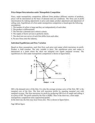
DD is the demand curve of the firm. It is also the average revenue curve of the firm. MC is the
marginal cost of the firm. The firm will maximise profits by equating marginal cost with
marginal revenue. The firm maximises its profit by producing OM level of output and selling it
at a price of OP. The profit earned by the firm is PQRS. Thus in the short run, a firm under
monopolistic competition earns supernormal profits.
In the short run, the firm may incur losses also. This is shown in figure below.
Page 188 last figure

2. The firm is in equilibrium by producing an output of OQ. It fixes the price at OP. As price is less
than cost, it incurs losses equal to PABC. Thus a firm in equilibrium under monopolistic
competition may be making supernormal profits or losses depending upon the position of the
demand curve and average cost curve.
Group Equilibrium and Price Variation
Group equilibrium refers to price-output determination in a number of firms whose products are
close substitutes. The product of each firm has special characteristics. The difference in the
quality of the products of the firms under monopolistic competition results in large variation in
elasticity and position of the demand curves of the various firms. Similarly the shape and
position of cost curves too differ. As a result there exist differences in prices, output and profits
of the various firms in the group. For the sake of simplicity in the analysis of group equilibrium,
Chamberlin ignores these differences by adopting infirmity assumption. He assumes that the cost
and demand curves of all the products in the group are uniform. Chamberlin introduces another
assumption known as 'symmetry assumption'. It means that the number of firms under
monopolistic competition is large and hence the action of an individual firm regarding price and
output will have a negligible effect upon his rivals.
Based on these assumptions, short run equilibrium of a firm under monopolistic competition can
be shown in Figure below:
Page 189 last figure
Figure (A) represents short run equilibrium and figures (B) the long run equilibrium. In the short
run, the price is OP and average cost is only MR. Hence there is supernormal profit equal to
PQRS. But in the long run, as shown in figure 27 (B), the excess profit is competed away. MC =
MR at OM level of output. LAR is tangent to LAC. Price is equal to average cost and there is no
extra profit. Only normal profit is earned.

3. PRODUCT DIFFERENTIATION
While analysing the equilibrium of a firm with regard to the variation of the product we assume
the price of product to be constant. The firm has to select among the various possible qualities
and attributes of the product. An important characteristic of product variation is that it changes
the cost curve and demand for the product. Therefore, the entrepreneur has to choose the product
whose cost and demand are such as to yield maximum profit. Yet another feature of product
variation is that product variation is qualitative and therefore, quantitative measurement is not
possible.
INDIVIDUAL EQUILIBRIUM AND PRODUCT VARIATION
The equilibrium of the firm under condition of product variation is shown in figure below:
Page 191 1st fig
AA is the average cost curve of the product A and BB is the average cost curve of the product B.
The price of the product is OP. If OM quantity of the product A is demanded at the price of OP,
the total costs are OMRS. The entrepreneur earns an abnormal profit equal to PQRS. If the
Quantity demanded of the product B is ON, then the total costs are ONFG and the total profits
made by the entrepreneur are GFEP. Since the product B yields greater profits than A, the
entrepreneur will select the product B.
Group Equilibrium and Product Variation
It is assumed that the demand is uniform and the possibility of product variation is also uniform.
The equilibrium adjustment of the product is shown in figure below:
CC1 is the average cost curve. If the quantity demanded is OM then the total cost is OMHG. The
firm earns supernormal profits equal to GHQP. This supernormal profits should be wiped away
to achieve group equilibrium. Attracted by the supernormal profits, new competitor may enter
the group. The quantity demanded will come down to OT.

4. Price will cover only cost of production. Besides, the adjustment in the number of firms, product
improvement may also take place. When all entrepreneurs improve their product, cost will
increase as shown by DD1 and become equal to the price at the point S.
Group equilibrium must satisfy the following conditions:
1. The average cost must be equal to price.
2. It is not possible for anyone to increase his profits by making further adjustment or
improvement in his product.
Selling Cost and Price Determination
Selling cost is another important factor which influences pricing under monopolistic competition.
Selling costs are costs incurred on advertising, publicity, salesmanship, free sampling, free
service, door to door canvassing and so on. Selling costs are "the costs necessary to persuade a
buyer to buy one product rather than another or to buy from one seller rather than another".
Under perfect competition, there is no need for advertising as the product is homogeneous.
Similarly, under monopoly also, selling costs are not needed as there are no rivals. But under
conditions of monopolistic competition, as the products are differentiated, selling costs are
essential to increase sales. Chamberlin defines selling cost as, "costs incurred in order to alter the
portion or shape of the demand curve for a product".
Advertisement may be classified into two types: informative and competitive. Informative
advertisement enables the buyers to know about existence and uses of the product. It also helps
to increase sales of all firms in the group. Competitive advertisement refers to expenses incurred
to increase the sales of the product of a particular firm as against other products.
Production cost versus selling cost
Though Watson feels that it is difficult to differentiate selling cost from cost of production,
Chamberlin states that these two costs are basically different from one another. Production costs
include all expenses incurred in producing a product and transporting it to its destination for
consumers. Selling costs are incurred to change the preferences of a consumer for a particular
product. Prof. Chamberlin distinguishes between the two in these words: "The former
(production) costs create utilities in order that demands may be satisfied; the latter create and
shift the demand curves themselves." Those which alter the demand curve for a product are
selling costs and those which do not are production costs. In other words, "those made to adapt
the product to the demand arc production costs and those made to adapt the demand to the
product are selling costs".
The production cost affects the supply but selling cost affects the demand. While the production
cost influences the volume of production, the selling cost influences the volume of sales. Selling
costs are subject to varying returns. When selling cost , increases, first it leads to increasing
returns and then to diminishing returns. Two factors are responsible for increasing returns.
1. Repeated and continuous advertisements bring in increasing returns. Advertisement seen
once will have negligible or no effect on consumer. Therefore, selling cost is a waste.

5. Continued advertising over a period of time and in different media brings favourable
effect.
2. Economies of large scale selling operations also lead to increasing returns. But as
advertising outlay increases, diminishing returns set in due to change in taste and preferences
of the people. Further, existing buyers may not increase their demand as a result of
advertisement. This is because as he buys more, utility falls. The effect of selling costs on the
demand for the product and the varying returns is shown in figure below:
page 194 1st figure
D1 is the demand curve before advertisement expenditure is incurred. When advertisement
expenditures are undertaken, the demand curve shifts to D2 D3 D4 and D5. At the price of OP,
quantity demanded increases from Ql toQ2, Q2 to Q3, Q3 to Q4 and Q4 to Q5. After D4,
diminishing returns occur.
The curve of selling cost is U-shaped, due to-the operation of the law of variable proportions.
The curve of selling cost first falls, reaches a minimum point and then starts rising as shown in
figure 31.
SC is the curve of selling costs. The total cost of selling OA units of the product is OAQS. At the
minimum point of the selling cost curve i.e. at M, the selling cost is the minimum. Beyond the
point M, selling cost increases. For instance, the average selling cost of OC is RC.
Individual Equilibrium and Selling Cost
Here it is assumed that the seller adjusts his selling cost keeping the price and product constant.
It is also assumed that one seller alone advertises, while all others do not. As a result he attracts
new buyers, sells more and makes profit. This is illustrated in figure 32.
Page 195 fig 31,32
PC is the production cost curve. CC1 is the combined production and selling cost curve. MC is
the marginal cost curve. If the seller sells OQ level of output at OP price, he has no profit. His
cost of production is equal to price. Therefore, he advertises his product which increases his cost.
His combined production and selling costs are indicated by CC1. At OQ1 level of output, his
production cost is equal to OQ1 S1 R1. His selling cost is R1 S1 SR. He earns an abnormal profit
equal to PRST.
Group Equilibrium and Selling Cost
The abnormal profit earned by the firm makes all other firms in the group advertise. When all
firms advertise total cost of all will increase. Price will be equal to cost. There is no abnormal
profit. All firms earn only normal profit. This is shown in figure below.

6. PC is the production cost curve. TC is the total cost curve of the single firm. Due to competition
from others, the cost is equal to price. CC is the total cost curve of all the firms in the group. As
it is tangent to the price, there is no abnormal profit.
Optimum Selling Costs
A producer undertakes advertisement only when it brings additional revenue. The producer will
increase his advertising expenditure as long as the marginal revenue is greater than marginal
cost. He will stop at the point at which marginal revenue is greater than marginal cost. He will
stop at the point at which marginal revenue is equal to marginal cost. Only at that point, profit
will be maximum. This is shown in figure below:
Page 197 1st fig
AR1 is the average revenue curve before advertisement. AC is the average cost curve. OP is the
price. The equilibrium level of output is OQ. If advertisement is undertaken, average revenue
curve will shift from AR1 to AR2 The average cost curve AC1 includes the cost of advertisement.
The equilibrium price will be OP1 and the output OQ1 Profits will be larger. Since profits have
increased the firm will continue its advertisement expenditure till the marginal revenue is equal
to marginal cost. Profit maximisation is achieved at OP2 price and OQ2 output. Beyond this
point, advertisement expenditure will lead to fall in profit. Therefore, a producer under
monopolistic competition has to select that cost and revenue curves where the profits are
maximum.
Duopoly
When there are two monopolists who share the monopoly power then it is called duopoly. It may
be of two types-duopoly without product differentiation and duopoly with product
differentiation. Under duopoly without product differentiation, there are two monopolists selling
an identical commodity. There is no product differentiation. There is also a possibility for
collusion. They may agree on price or divide the market for goods. Suppose, if there is no
agreement between the two, a constant price war will emerge. In this case they will earn only

7. normal profits. If their costs are different, the one with lower costs will squeeze out the other and
a simple monopoly would result. The best course for the duopolists will be to fix the monopoly
price and share the market and profits. In the. short run, duopoly price may be lower than the
competitive price. In the long run, the price maybe somewhere between the monopoly price and
the competitive price. When there is product differentiation, each producer will have his own
customers. There is no danger of price war. There is no agreement. Since products are
differentiated the firm with better product will earn supernormal profits.
OLIGOPOLY
Oligopoly is a situation in which few large firms compete against each other and there is an
element of interdependence in the decision making of these firms. A policy change on the part of
one firm will have immediate effects on competitors, who react with their counter policies.
Features
Following are the features of oligopoly which distinguish it from .other market structures :
1. Small number of large sellers:
The number of sellers dealing in a homogeneous or differentiated product is small. The policy of
one seller will have a noticeable impact on market, mainly on price and output.
2. Interdependence:
Unlike perfect competition and monopoly, the oligopolist is not independent to take decisions.
The oligopolist has to take into account the actions and reactions of his rivals while deciding his
price and output policies. As the products of the oligopolist are close substitutes, the cross
elasticity of demand is very high.
3. Price rigidity:
Any change in price by one oligopolist invites retaliation and counter- action from others, the
oligopolist normally sticks to one price. If an oligopolist reduces his price, his rivals will also do
so and therefore, it is not advantageous for the oligopolist to reduce the price. On the other hand,
if an oligopolist tries to raise the price, others will not do so. As a result they capture the
customers of this firm. Hence the oligopolist would never try to either reduce or raise the price.
This results in price rigidity.
4. Monopoly element:
As products are differentiated the firms enjoy some monopoly power. Further, when firms
collude with each other, they can work together to raise the price and earn some monopoly
income.
5. Advertising:
The only way open to the oligopolists to raise his sales is either by advertising or improving the
quality of the product. Advertisement expenditure is used as an effective tool to shift the demand
in favour of the product. Quality improvement will also shift the demand favorably. Usually,

8. both advertisements as well as variations in designs and quality are used simultaneously to
maintain and increase the market share of an oligopolist.
6. Group behavior:
The firms under oligopoly recognise their interdependence and realise the importance of mutual
cooperation. Therefore, there is a tendency among them for collusion. Collusion as well as
competition prevails in the oligopolistic market leading to uncertainty and indeterminateness.
7. Indeterminate demand curve:
It is not possible for an oligopolist to forecast the nature and position of the demand curve with
certainty. The firm cannot estimate the sales when it decides to reduce the price. Hence the
demand curve under oligopoly is indeterminate.
TYPES OF OLIGOPOLY:
Oligopoly may be classified in the following ways:
a. Perfect and imperfect oligopoly.
On the basis of the nature of product, oligopoly may be classified into perfect (pure) and
imperfect (differentiated) oligopoly. If the products are homogeneous, then oligopoly is called as
perfect or pure oligopoly. If the products are differentiated and are close substitutes, then it is
called as imperfect or differentiated oligopoly.
b. Open or closed oligopoly.
On the basis of possibility of entry of new firms, oligopoly may be classified into open or closed
oligopoly. When new firms are free to enter, it is open oligopoly. When few firms dominate the
market and new firms do not have a free entry into the industry, it is called closed oligopoly.
c. Partial and full oligopoly.
Partial oligopoly refers to a situation where one firm acts as the leader and others follow it. On
the other hand, full oligopoly exists where no firm is dominating as the price leader.
d. Collusive and non- collusive oligopoly.
Instead of competition with each other, if the firms follow a common price policy, it is called
collusive oligopoly. If the collusion is in the form of an agreement, it is called open collusion. If
it is an understanding between the firms, then it is a secret collusion. On the other hand, if there
is no agreement or understanding between oligopoly firms, it is known as non-collusive
oligopoly.
e. Syndicated and organised oligopoly:
Syndicated oligopoly is one in which the firms sell their products through a centralised
syndicate. Organised oligopoly refers to the situation where the firms organize themselves into a
central association for fixing prices, output, quota etc.

9. MODELS OF OLIGOPOLY
1. Cournot's model of oligopoly: Augustin Cournot, a French economist, published his
Theory of duopoly in 1838. Cournot dealt with a case of duopoly. He has taken the case of
two identical mineral springs operated by two owners. His model is based on the following
assumptions:
1. The product is homogenous.
2. There is no cost of production. The average cost and marginal cost are zero.
3. Output of the rival is assumed to be constant.
4. The market demand for the product is linear.
DB is the market demand curve. OB is the total quantity of mineral water which can be produced
and supplied by the two producers. If both the producers produce the maximum quantity of OB,
the price will be zero. This is because cost of production is assumed to be zero. Cournot assumes
that one producer say X starts production first. He will produce OA output and his profit will be
OAPK. Suppose the second producer Y enters into the market. He assumes that the first producer
will continue to produce the same. So Y considers PB as his demand curve. With this demand
curve, he will produce AH amount of output. The total output will now be OA + AH = OH and
the price will fall to OF. The total profits for both the producers will be OHQR. Out of these total
profits, producers X will get OAGF and Y will receive AHQG. Now that the profits of producers
X are reduced from OAPK to OAGF by producers Y producing AH output, producer X will
reconsider the situation. But he will assume that producer Y will continue to produce AH output.
Therefore, he reduces his output from OA to OT. Now the total output will be OT + AH = ON
and the price will be OS and the total profits of the two will be ONRS. Out of the total profits, X
will get OTLS and Y will get TNRL. Now the producer Y will reappraise his situation. Believing
that producer X will continue producing OT, the producer Y will find his maximum profits by
producing output equal to 1/2 TB. With this move of producer Y, producer X will find his profits
reduced. Therefore, X will reconsider his position. This process of adjustment and readjustment
by each producer will continue, until the total output OM is produced and each is producing the
same amount of output. In the final position, producer X produces OC amount of output and
producer Y produces CM amount of output and OC = CM.
Cournot's duopoly solution can be extended to a situation with more than two sellers. If there
were three producers, the total output would be 3/4 of OB, each producing 1/4 OB. If there are n
producers, then under Cournot's solutions, the total output produced will be (n 1)/n of OB

10. where OB is the maximum possible output. The essential conclusion is that; as the number of
sellers increases from one to infinity the price is continually lowered from what it would be
under monopoly conditions to what it would be under purely competitive conditions, and that for
any number of sellers, it is perfectly determinate. The basic weakness of Cournot's duopoly
model is that the rivals assume the output of the other to be fixed, even though they observe
constant changes in output.
2. Bertrand's model
Joseph Bertrand, a French mathematician criticised Cournot's duopoly solution and put forward a
substitute model of oligopoly. In Bertrand's model, each producer assumes his rival's price to be
constant. The products produced and sold by the two producers are completely identical. The two
producers have identical costs. Moreover, the productive capacity of the producers is unlimited.
Bertrand's model can be explained with an example. There are two producers A and B. If A goes
into business first, he will set the price at the monopoly level, which is the most profitable for
him. Suppose B also enters into the business and starts producing the same product as produced
by A. B assume that A will go on charging the same price Therefore, he can undercut the price
changed by A to capture the whole market. He will set a price slightly lower than I A's price. A's
sales fall to zero. Now A will reconsider his price policy. He assumes that, B will continue to
charge the same price. There are two alternatives open to him. First, he may match the price cut
made by B or he may charge the same price as B charges. In this case, he will secure half the
market. Secondly, he may undercut B and set a slightly lower price than that of B. In this case A
will seize the entire market. Evidently the latter course looks more profitable and thus A
undercuts B and sets a price lower than B's price. Now producer B will react and think of
changing his price, He also has two alternatives: He may match A's price or undercut him. Since
undercutting is more profitable, B will set a price a little lower than A and seize the whole
market. But again A will be forced to undercut B. This price war will go on until price falls to the
level of cost. When price is equal to cost, neither of them will like to cut the price further or raise
the price and therefore, the equilibrium has been achieved. In Bertrand’s model, equilibrium is
achieved when market price is equal to the average cost of production and the combined
equilibrium output of the two duopolies is equal to the competitive output.
3. Edge worth model
F.Y. Edge worth, a famous French economist, also attacked Cournot's duopoly solution. He
criticised 'Cournot's assumption that each duopolist believes that his rival will continue to
produce the same output irrespective of what he himself might produce. According to Edge
worth each duopolist believes that his rival will continue to charge the same price. With this
assumption and taking the example of Cournot's "mineral wells", Edge worth showed that no
determinate equilibrium would be reached in duopoly. Further, it is also assumed that the
products of the two duopolists are perfectly homogeneous. The cost conditions of the two
duopolists need not be exactly same but must be similar. Edge worth’s model is given in figure
below:
Page 206 1st fig
AB is the demand curve for producer X and AB1 is the demand curve for producer Y. The
maximum possible quantity each producer can produce and supply is OQ by X and OQ1 by Y. If

11. each producer wants to sell his entire output, he will have to fix the price as OP1 On the other
hand, if the two rivals join together to maximise profit, they will fix the price at OP and sell ON
and ON1 output respectively. Each producer will get a maximum profit of ONCP and ON1 C1P
respectively.
To start with, if the two producers charge the price OP then X and Y will be selling ON and ON 1
amounts of output respectively. Suppose producer X thinks of revising his price policy. Producer
X will believe that producer Y will keep his price unchanged at OP. He realises that if he sets the
price slightly lower than OP he can sell his entire output and get maximum profit. So producer X
will lower his price from OP to OR and sells his entire output OQ and will earn profits equal to
OQSR. This X would increase his profit by lowering his price.
But when producer X reduces his price, producer Y will find his sales considerably reduced.
Profits will fall. As a result, producer Y will fix price at OR1 so that he can sell his entire output.
As a result of this, sales and profits of producer X will greatly decline. Producer X will now react
and will think that if he reduces his price a little below OR1 he will be able to sell his whole
output by attracting customers of producer Y. Thus when producer X reduces his price, his
profits will increase for a moment. But producer Y will react and reduce his price further to
increase his profits. In this way, price cutting will continue until the price falls to the level OP 1 at
which both producers sell their entire output. At OP1, producers X and Y are selling OB and OB1
respectively and are making profits equal to OBTP1 and OB1T1P1 respectively. According to
Edge worth, equilibrium is not attained at OP1 price. Each will have incentive to raise the price.
If producer X raises the price to OP, he will earn ONCP which are larger than profits at OP 1
price. Producer Y will also raise his price to the level slightly lower than OP. Producer X will
now fix the price slightly lower than Y's level. In this way, price will fluctuate between OP and
OP1 gradually downwards but upwards in a jump. Thus Edge worth’s duopoly solution is one of
perpetual disequilibrium and price will be constantly oscillating between the monopoly price and
competitive price. No determinate and unique equilibrium of duopoly is suggested by Edge
worth’s duopoly model.
4. Chamberlin's Duopoly Model
Edward Chamberlin has modified Cournot's model by assuming that the rivals understand the
reality. His model is same as that of Cournot's. AB is the market demand for mineral water. If
producer X enters the market first, he will produce ON quantity at OP price and secure
maximum monopoly profit of ONCP. At this stage producer Y enters the market and produces
NQ amount and fixes OP' price and gets a profit of NQDE. Upto this point Chamberlin's analysis
is the same as Cournot's.

12. From this point onwards, Chamberlin's analysis is different. Producer X immediately realises the
mutual interdependence of the two producers and he reduces his output from ON to OM.
Producer Y will produce the same amount NQ. Thus both produce the monopoly output of ON,
fix the monopoly price OP and share equally the monopoly profit. (OMLP for X and MNCL for
Y). Under this system there is stability but in Edge worth’s duopoly solution there is instability.
Besides Chamberlin's model is a realistic description of the actual duopoly market situation.
Sweezy's Model
P. Sweezy introduced the kinked demand curve to explain the determination of equilibrium in'
oligopolistic market. The demand curve facing an oligopolist has a kink at the prevailing price.
This is because each oligopolist believes that if he lowers the price below the prevailing level
increases his price above the prevailing level his competitors will not follow his increase in price.
Due to this behavioural pattern of the oligopolists, the upper segment of the demand curve is
relatively elastic and the lower portion is relatively inelastic.
Page 209 1st fig
If the oligopolist reduces its price below the prevailing price level MP, the competitors will fear
that their customers would go away from them. Therefore, they will also reduce the price. Since
all the competitors are reducing their price, the oligopolist will gain only very little sales. Hence
the demand curve which lies below the prevailing price is inelastic. If the oligopolist raises his
price above the prevailing price level his sales will be reduced. As a result of a rise in price, his
customers will go to his competitors.

13. Thus an increase in price will lead to a large reduction in sales. This shows that the demand
curve which lies above the current price level is elastic. Since the oligopolist will not gain a
larger share of the market by reducing his price below the prevailing level and will loose a large
share of the market by increasing his price he will not change the price. For determining profit
maximising price-output, combination, marginal revenue curve has to be drawn. The marginal
revenue curve corresponding to the kinked demand curve has a gap or discontinuity between G
and H. This gap in MR curve occurs due to the kink in the demand curve and lies right below the
kink. The length of the gap depends on the relative elasticities of the two portions of the demand
curve. The greater the difference in the two elasticities the greater the length of the discontinuity.
If the marginal cost curve of the oligopolist passes through the discontinuous portion of the MR
curve the oligopolist will be maximising his profit at the prevailing price level OP. As he is
maximising profits at the prevailing price level he will have no incentive to change the price.
Even if cost conditions change the price will remain stable.
Page 210 1st fig
When the marginal cost curve shifts upward from MC to MC1 , the price remains unchanged as
MC1 passes through the gap GH. Similarly, the price will remain stable even when the demand
conditions change. When the demand for the oligopolist increases from D to D1, the given
marginal cost curve MC cuts the new marginal revenue curve MR within the gap. This means
that the same price continues to prevail in the market.
The major drawback of the kinked demand curve is that it does not explain the determination of
price. It explains only price rigidity. Further it is not applicable to price leadership and cartels.
Kinked demand curve is also not applicable to oligopoly with product differentiation. Due to
these deficiencies, a general theory of pricing is impossible under oligopoly.