5. CHAPTER 1: Introduction
EXERCISES 1.1: Background, page 5
1. This equation involves only ordinary derivatives of x with respect to t, and the highest deriva-
tive has the second order. Thus it is an ordinary differential equation of the second order with
independent variable t and dependent variable x. It is linear because x, dx/dt, and d2
x/dt2
appear in additive combination (even with constant coefficients) of their first powers.
3. This equation is an ODE because it contains no partial derivatives. Since the highest order
derivative is dy/dx, the equation is a first order equation. This same term also shows us that
the independent variable is x and the dependent variable is y. This equation is nonlinear
because of the y in the denominator of the term [y(2 − 3x)]/[x(1 − 3y)] .
5. This equation is an ODE because it contains only ordinary derivatives. The term dp/dt is the
highest order derivative and thus shows us that this is a first order equation. This term also
shows us that the independent variable is t and the dependent variable is p. This equation
is nonlinear since in the term kp(P − p) = kPp − kp2
the dependent variable p is squared
(compare with equation (7) on page 5 of the text).
7. This equation is an ordinary first order differential equation with independent variable x and
dependent variable y. It is nonlinear because it contains the square of dy/dx.
9. This equation contains only ordinary derivative of y with respect to x. Hence, it is an ordi-
nary differential equation of the second order (the highest order derivative is d2
y/dx2
) with
independent variable x and dependent variable y. This equation is of the form (7) on page 5
of the text and, therefore, is linear.
1
6. Chapter 1
11. This equation contains partial derivatives, thus it is a PDE. Because the highest order deriva-
tive is a second order partial derivative, the equation is a second order equation. The terms
∂N/∂t and ∂N/∂r show that the independent variables are t and r and the dependent variable
is N.
13. Since the rate of change of a quantity means its derivative, denoting the coefficient propor-
tionality between dp/dt and p(t) by k (k > 0), we get
dp
dt
= kp.
15. In this problem, T ≥ M (coffee is hotter than the air), and T is a decreasing function of t,
that is dT/dt ≤ 0. Thus
dT
dt
= k(M − T),
where k > 0 is the proportionality constant.
17. In classical physics, the instantaneous acceleration, a, of an object moving in a straight line
is given by the second derivative of distance, x, with respect to time, t; that is
d2
x
dt2
= a.
Integrating both sides with respect to t and using the given fact that a is constant we obtain
dx
dt
= at + C. (1.1)
The instantaneous velocity, v, of an object is given by the first derivative of distance, x,
with respect to time, t. At the beginning of the race, t = 0, both racers have zero velocity.
Therefore we have C = 0. Integrating equation (1.1) with respect to t we obtain
x =
1
2
at2
+ C1 .
For this problem we will use the starting position for both competitors to be x = 0 at t = 0.
Therefore, we have C1 = 0. This gives us a general equation used for both racers as
x =
1
2
at2
or t =
2x
a
,
2
7. Exercises 1.2
where the acceleration constant a has different values for Kevin and for Alison. Kevin covers
the last 1
4
of the full distance, L, in 3 seconds. This means Kevin’s acceleration, aK, is
determined by:
tK − t3/4 = 3 =
2L
aK
−
2(3L/4)
aK
,
where tK is the time it takes for Kevin to finish the race. Solving this equation for aK gives,
aK =
√
2 − 3/2
2
9
L.
Therefore the time required for Kevin to finish the race is given by:
tK =
2L
√
2 − 3/2
2
L/9
=
3
√
2 − 3/2
√
2 = 12 + 6
√
3 ≈ 22.39 sec.
Alison covers the last 1/3 of the distance, L, in 4 seconds. This means Alison’s acceleration,
aA, is found by:
tA − t2/3 = 4 =
2L
aA
−
2(2L/3)
aA
,
where tA is the time required for Alison to finish the race. Solving this equation for aA gives
aA =
√
2 − 4/3
2
16
L.
Therefore the time required for Alison to finish the race is given by:
tA =
2L
√
2 − 4/3
2
(L/16)
=
4
√
2 − 4/3
√
2 = 12 + 4
√
6 ≈ 21.80 sec.
The time required for Alison to finish the race is less than Kevin; therefore Alison wins the
race by 6
√
3 − 4
√
6 ≈ 0.594 seconds.
EXERCISES 1.2: Solutions and Initial Value Problems, page 14
1. (a) Differentiating φ(x) yields φ (x) = 6x2
. Substitution φ and φ for y and y into the given
equation, xy = 3y, gives
x 6x2
= 3 2x3
,
3
8. Chapter 1
which is an identity on (−∞, ∞). Thus φ(x) is an explicit solution on (−∞, ∞).
(b) We compute
dφ
dx
=
d
dx
(ex
− x) = ex
− 1.
Functions φ(x) and φ (x) are defined for all real numbers and
dφ
dx
+φ(x)2
= (ex
− 1)+(ex
− x)2
= (ex
− 1)+ e2x
− 2xex
+ x2
= e2x
+(1−2x)ex
+x2
−1,
which is identically equal to the right-hand side of the given equation. Thus φ(x) is an
explicit solution on (−∞, ∞).
(c) Note that the function φ(x) = x2
− x−1
is not defined at x = 0. Differentiating φ(x)
twice yields
dφ
dx
=
d
dx
x2
− x−1
= 2x − (−1)x−2
= 2x + x−2
;
d2
φ
dx2
=
d
dx
dφ
dx
=
d
dx
2x + x−2
= 2 + (−2)x−3
= 2 1 − x−3
.
Therefore
x2 d2
φ
dx2
= x2
· 2 1 − x−3
= 2 x2
− x−1
= 2φ(x),
and φ(x) is an explicit solution to the differential equation x2
y = 2y on any interval not
containing the point x = 0, in particular, on (0, ∞).
3. Since y = sin x+x2
, we have y = cos x+2x and y = − sin x+2. These functions are defined
on (−∞, ∞). Substituting these expressions into the differential equation y + y = x2
+ 2
gives
y + y = − sin x + 2 + sin x + x2
= 2 + x2
= x2
+ 2 for all x in (−∞, ∞).
Therefore, y = sin x + x2
is a solution to the differential equation on the interval (−∞, ∞).
5. Differentiating x(t) = cos 2t, we get
dx
dt
=
d
dt
(cos 2t) = (− sin 2t)(2) = −2 sin 2t.
4
9. Exercises 1.2
So,
dx
dt
+ tx = −2 sin 2t + t cos 2t ≡ sin 2t
on any interval. Therefore, x(t) is not a solution to the given differential equation.
7. We differentiate y = e2x
− 3e−x
twice:
dy
dx
=
d
dx
e2x
− 3e−x
= e2x
(2) − 3e−x
(−1) = 2e2x
+ 3e−x
;
d2
y
dx2
=
d
dx
dy
dx
=
d
dx
2e2x
+ 3e−x
= 2e2x
(2) + 3e−x
(−1) = 4e2x
− 3e−x
.
Substituting y, y , and y into the differential equation and collecting similar terms, we get
d2
y
dx2
−
dy
dx
− 2y = 4e2x
− 3e−x
− 2e2x
+ 3e−x
− 2 e2x
− 3e−x
= (4 − 2 − 2)e2x
+ (−3 − 3 − 2(−3))e−x
= 0.
Hence y = e2x
− 3e−x
is an explicit solution to the given differential equation.
9. Differentiating the equation x2
+ y2
= 6 implicitly, we obtain
2x + 2yy = 0 ⇒ y = −
x
y
.
Since there can be no function y = f(x) that satisfies the differential equation y = x/y and
the differential equation y = −x/y on the same interval, we see that x2
+ y2
= 6 does not
define an implicit solution to the differential equation.
11. Differentiating the equation exy
+ y = x − 1 implicitly with respect to x yields
d
dx
(exy
+ y) =
d
dx
(x − 1)
⇒ exy d
dx
(xy) +
dy
dx
= 1
⇒ exy
y + x
dy
dx
+
dy
dx
= 1
⇒ yexy
+
dy
dx
(xexy
+ 1) = 1
⇒
dy
dx
=
1 − yexy
1 + xexy
=
exy
(e−xy
− y)
exy (e−xy + x)
=
e−xy
− y
e−xy + x
.
5
10. Chapter 1
Therefore, the function y(x) defined by exy
+ y = x − 1 is an implicit solution to the given
differential equation.
13. Differentiating the equation sin y + xy − x3
= 2 implicitly with respect to x, we obtain
y cos y + xy + y − 3x2
= 0
⇒ (cos y + x)y = 3x2
− y ⇒ y =
3x2
− y
cos y + x
.
Differentiating the second equation above again, we obtain
(−y sin y + 1)y + (cos y + x)y = 6x − y
⇒ (cos y + x)y = 6x − y + (y )2
sin y − y = 6x − 2y + (y )2
sin y
⇒ y =
6x − 2y + (y )2
sin y
cos y + x
.
Multiplying the right-hand side of this last equation by y /y = 1 and using the fact that
y =
3x2
− y
cos y + x
,
we get
y =
6x − 2y + (y )2
sin y
cos y + x
·
y
(3x2 − y)/(cos y + x)
=
6xy − 2(y )2
+ (y )3
sin y
3x2 − y
.
Thus y is an implicit solution to the differential equation.
15. We differentiate φ(x) and substitute φ and φ into the differential equation for y and y . This
yields
φ(x) = Ce3x
+ 1 ⇒
dφ(x)
dx
= Ce3x
+ 1 = 3Ce3x
;
dφ
dx
− 3φ = 3Ce3x
− 3 Ce3x
+ 1 = (3C − 3C)e3x
− 3 = −3,
which holds for any constant C and any x on (−∞, ∞). Therefore, φ(x) = Ce3x
+ 1 is a
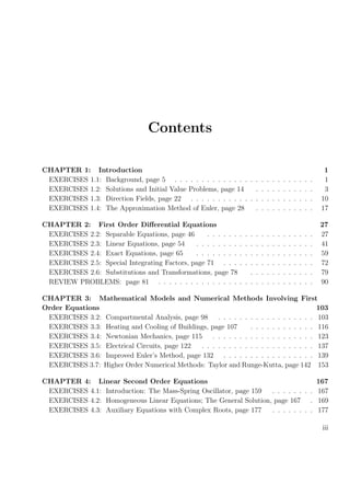
one-parameter family of solutions to y −3y = −3 on (−∞, ∞). Graphs of these functions for
C = 0, ±0.5, ±1, and ±2 are sketched in Figure 1-A.
6
11. Exercises 1.2
–10
10
–0.5 0.5
C=2
C=1
C=0.5
C=0
C=−0.5
C=−1
C=−2
Figure 1–A: Graphs of the functions y = Ce3x
+ 1 for C = 0, ±0.5, ±1, and ±2.
17. Differentiating φ(x), we find that
φ (x) =
2
1 − cex
= 2 (1 − cex
)−1
= 2(−1) (1 − cex
)−2
(1 − cex
) = 2cex
(1 − cex
)−2
. (1.2)
On the other hand, substitution of φ(x) for y into the right-hand side of the given equation
yields
φ(x)(φ(x) − 2)
2
=
1
2
2
1 − cex
2
1 − cex
− 2
=
2
1 − cex
1
1 − cex
− 1 =
2
1 − cex
1 − (1 − cex
)
1 − cex
=
2cex
(1 − cex)2
,
which is identical to φ (x) found in (1.2).
19. Squaring and adding the terms dy/dx and y in the equation (dy/dx)2
+ y2
+ 3 = 0 gives a
nonnegative number. Therefore when these two terms are added to 3, the left-hand side will
always be greater than or equal to three and hence can never equal the right-hand side which
is zero.
7
12. Chapter 1
21. For φ(x) = xm
, we have φ (x) = mxm−1
and φ (x) = m(m − 1)xm−2
.
(a) Substituting these expressions into the differential equation, 3x2
y + 11xy − 3y = 0,
gives
3x2
m(m − 1)xm−2
+ 11x mxm−1
− 3xm
= 0
⇒ 3m(m − 1)xm
+ 11mxm
− 3xm
= 0
⇒ [3m(m − 1) + 11m − 3] xm
= 0
⇒ 3m2
+ 8m − 3 xm
= 0.
For the last equation to hold on an interval for x, we must have
3m2
+ 8m − 3 = (3m − 1)(m + 3) = 0.
Thus either (3m − 1) = 0 or (m + 3) = 0, which gives m =
1
3
, −3.
(b) Substituting the above expressions for φ(x), φ (x), and φ (x) into the differential equa-
tion, x2
y − xy − 5y = 0, gives
x2
m(m − 1)xm−2
− x mxm−1
− 5xm
= 0 ⇒ m2
− 2m − 5 xm
= 0.
For the last equation to hold on an interval for x, we must have
m2
− 2m − 5 = 0.
To solve for m we use the quadratic formula:
m =
2 ±
√
4 + 20
2
= 1 ±
√
6 .
23. In this problem, f(x, y) = x3
− y3
and so
∂f
∂y
=
∂ (x3
− y3
)
∂y
= −3y2
.
Clearly, f and ∂f/∂y (being polynomials) are continuous on the whole xy-plane. Thus the
hypotheses of Theorem 1 are satisfied, and the initial value problem has a unique solution for
any initial data, in particular, for y(0) = 6.
8
13. Exercises 1.2
25. Writing
dx
dt
= −
4t
x
= −4tx−1
,
we see that f(t, x) = −4tx−1
and ∂f(t, x)/∂x = ∂(−4tx−1
)/∂x = 4tx−2
. The functions
f(t, x) and ∂f(t, x)/∂x are not continuous only when x = 0. Therefore, they are continuous
in any rectangle R that contains the point (2, −π), but does not intersect the t-axis; for
instance, R = {(t, x) : 1 < t < 3, −2π < x < 0}. Thus, Theorem 1 applies, and the given
initial problem has a unique solution.
26. Here f(x, y) = 3x − 3
√
y − 1 and ∂f(x, y)/∂y = −1
3
(y − 1)−2/3
. Unfortunately, ∂f/∂y is not
continuous or defined when y = 1. So there is no rectangle containing (2, 1) in which both f
and ∂f/∂y are continuous. Therefore, we are not guaranteed a unique solution to this initial
value problem.
27. Rewriting the differential equation in the form dy/dx = x/y, we conclude that f(x, y) = x/y.
Since f is not continuous when y = 0, there is no rectangle containing the point (1, 0) in
which f is continuous. Therefore, Theorem 1 cannot be applied.
29. (a) Clearly, both functions φ1(x) ≡ 0 and φ2(x) = (x − 2)3
satisfy the initial condition,
y(2) = 0. Next, we check that they also satisfy the differential equation dy/dx = 3y2/3
.
dφ1
dx
=
d
dx
(0) = 0 = 3φ1(x)2/3
;
dφ2
dx
=
d
dx
(x − 2)3
= 3(x − 2)2
= 3 (x − 2)3 2/3
= 3φ2(x)2/3
.
Hence both functions, φ1(x) and φ2(x), are solutions to the initial value problem of
Exapmle 9.
(b) In this initial value problem,
f(x, y) = 3y2/3
⇒
∂f(x, y)
∂y
= 3
2
3
y2/3−1
=
2
y1/3
,
x0 = 0 and y0 = 10−7
. The function f(x, y) is continuous everywhere; ∂f(x, y)/∂y is
continuous in any region which does not intersect the x-axis (where y = 0). In particular,
9
14. Chapter 1
both functions, f(x, y) and ∂f(x, y)/∂y, are continuous in the rectangle
R = (x, y) : −1 < x < 1, (1/2)10−7
< y < (2)10−7
containing the initial point (0, 10−7
). Thus, it follows from Theorem 1 that the given
initial value problem has a unique solution in an interval about x0.
31. (a) To try to apply Theorem 1 we must first write the equation in the form y = f(x, y).
Here f(x, y) = 4xy−1
and ∂f(x, y)/∂y = −4xy−2
. Neither f nor ∂f/∂y are continuous
or defined when y = 0. Therefore there is no rectangle containing (x0, 0) in which both
f and ∂f/∂y are continuous, so Theorem 1 cannot be applied.
(b) Suppose for the moment that there is such a solution y(x) with y(x0) = 0 and x0 = 0.
Substituting into the differential equation we get
y(x0)y (x0) − 4x0 = 0 (1.3)
or
0 · y (x0) − 4x0 = 0 ⇒ 4x0 = 0.
Thus x0 = 0, which is a contradiction.
(c) Taking C = 0 in the implicit solution 4x2
− y2
= C given in Example 5 on page 9 gives
4x2
− y2
= 0 or y = ±2x. Both solutions y = 2x and y = −2x satisfy y(0) = 0.
EXERCISES 1.3: Direction Fields, page 22
1. (a) For y = ±2x,
dy
dx
=
d
dx
(±2x) = ±2 and
4x
y
=
4x
±2x
= ±2, x = 0.
Thus y = 2x and y = −2x are solutions to the differential equation dy/dx = 4x/y on
any interval not containing the point x = 0.
(b) , (c) See Figures B.1 and B.2 in the answers of the text.
10
15. Exercises 1.3
(d) As x → ∞ or x → −∞, the solution in part (b) increases unboundedly and has the lines
y = 2x and y = −2x, respectively, as slant asymptotes. The solution in part (c) also
increases without bound as x → ∞ and approaches the line y = 2x, while it is not even
defined for x < 0.
3. From Figure B.3 in the answers section of the text, we conclude that, regardless of the initial
velocity, v(0), the corresponding solution curve v = v(t) has the line v = 8 as a horizontal
asymptote, that is, limt→∞ v(t) = 8. This explains the name “terminal velocity” for the value
v = 8.
5. (a) The graph of the directional field is shown in Figure B.4 in the answers section of the
text.
(b), (c) The direction field indicates that all solution curves (other than p(t) ≡ 0) will approach
the horizontal line (asymptote) p = 1.5 as t → +∞. Thus limt→+∞ p(t) = 1.5 .
(d) No. The direction field shows that populations greater than 1500 will steadily decrease,
but can never reach 1500 or any smaller value, i.e., the solution curves cannot cross
the line p = 1.5 . Indeed, the constant function p(t) ≡ 1.5 is a solution to the given
logistic equation, and the uniqueness part of Theorem 1, page 12, prevents intersections
of solution curves.
6. (a) The slope of a solution to the differential equation dy/dx = x + sin y is given by dy/dx .
Therefore the slope at (1, π/2) is equal to
dy
dx
= 1 + sin
π
2
= 2.
(b) The solution curve is increasing if the slope of the curve is greater than zero. From part
(a) we know the slope to be x + sin y. The function sin y has values ranging from −1 to
1; therefore if x is greater than 1 then the slope will always have a value greater than
zero. This tells us that the solution curve is increasing.
(c) The second derivative of every solution can be determined by finding the derivative of
11
16. Chapter 1
the differential equation dy/dx = x + sin y. Thus
d
dx
dy
dx
=
d
dx
(x + sin y);
⇒
d2
y
dx2
= 1 + (cos y)
dy
dx
(chain rule)
= 1 + (cos y)(x + sin y) = 1 + x cos y + sin y cos y;
⇒
d2
y
dx2
= 1 + x cos y +
1
2
sin 2y.
(d) Relative minima occur when the first derivative, dy/dx, is equal to zero and the second
derivative, d2
y/dx2
, is greater than zero. The value of the first derivative at the point
(0, 0) is given by
dy
dx
= 0 + sin 0 = 0.
This tells us that the solution has a critical point at the point (0, 0). Using the second
derivative found in part (c) we have
d2
y
dx2
= 1 + 0 · cos 0 +
1
2
sin 0 = 1.
This tells us the point (0, 0) is a relative minimum.
7. (a) The graph of the directional field is shown in Figure B.5 in the answers section of the
text.
(b) The direction field indicates that all solution curves with p(0) > 1 will approach the
horizontal line (asymptote) p = 2 as t → +∞. Thus limt→+∞ p(t) = 2 when p(0) = 3.
(c) The direction field shows that a population between 1000 and 2000 (that is 1 < p(0) < 2)
will approach the horizontal line p = 2 as t → +∞.
(d) The direction field shows that an initial population less than 1000 (that is 0 ≤ p(0) < 1)
will approach zero as t → +∞.
(e) As noted in part (d), the line p = 1 is an asymptote. The direction field indicates that a
population of 900 (p(0) = 0.9) steadily decreases with time and therefore cannot increase
to 1100.
12
17. Exercises 1.3
9. (a) The function φ(x), being a solution to the given initial value problem, satisfies
dφ
dx
= x − φ(x), φ(0) = 1. (1.4)
Thus
d2
φ
dx2
=
d
dx
dφ
dx
=
d
dx
(x − φ(x)) = 1 −
dφ
dx
= 1 − x + φ(x),
where we have used (1.4) substituting (twice) x − φ(x) for dφ/dx.
(b) First we note that any solution to the given differential equation on an interval I is
continuously diferentiable on I. Indeed, if y(x) is a solution on I, then y (x) does exist
on I, and so y(x) is continuous on I because it is differentiable. This immediately implies
that y (x) is continuous as the difference of two continuous functions, x and y(x).
From (1.4) we conclude that
dφ
dx x=0
= [x − φ(x)] x=0
= 0 − φ(0) = −1 < 0
and so the continuity of φ (x) implies that, for |x| small enough, φ (x) < 0. By the
Monotonicity Test, negative derivative of a function results that the function itself is
decreasing.
When x increases from zero, as far as φ(x) > x, one has φ (x) < 0 and so φ(x) decreases.
On the other hand, the function y = x increases unboundedly, as x → ∞. Thus, by
intermediate value theorem, there is a point, say, x∗
> 0, where the curve y = φ(x)
crosses the line y = x. At this point, φ(x∗
) = x∗
and hence φ (x∗
) = x∗
− φ(x∗
) = 0.
(c) From (b) we conclude that x∗
is a critical point for φ(x) (its derivative vanishes at this
point). Also, from part (a), we see that
φ (x∗
) = 1 − φ (x∗
) = 1 > 0.
Hence, by Second Derivative Test, φ(x) has a relative minimum at x∗
.
(d) Remark that the arguments, used in part (c), can be applied to any point x, where
φ (x) = 0, to conclude that φ(x) has a relative minimum at x. Since a continuously
13
18. Chapter 1
differentiable function on an interval cannot have two relative minima on an interval
without having a point of relative maximum, we conclude that x∗
is the only point where
φ (x) = 0. Continuity of φ (x) implies that it has the same sign for all x > x∗
and,
therefore, it is positive there since it is positive for x > x∗
and close to x∗
(φ (x∗
) = 0
and φ (x∗
) > 0). By Monotonicity Test, φ(x) increases for x > x∗
.
(e) For y = x − 1, dy/dx = 1 and x − y = x − (x − 1) = 1. Thus the given differential
equation is satisfied, and y = x − 1 is indeed a solution.
To show that the curve y = φ(x) always stays above the line y = x − 1, we note that the
initial value problem
dy
dx
= x − y, y(x0) = y0 (1.5)
has a unique solution for any x0 and y0. Indeed, functions f(x, y) = x−y and ∂f/∂y ≡ −1
are continuous on the whole xy-plane, and Theorem 1, Section 1.2, applies. This implies
that the curve y = φ(x) always stays above the line y = x − 1:
φ(0) = 1 > −1 = (x − 1) x=0
,
and the existence of a point x with φ (x) ≤ (x − 1) would imply, by intermediate value
theorem, the existence of a point x0, 0 < x0 ≤ x, satisfying y0 := φ(x0) = x0 − 1 and,
therefore, there would be two solutions to the initial value problem (1.5).
Since, from part (a), φ (x) = 1−φ (x) = 1−x+φ(x) = φ(x)−(x−1) > 0, we also conclude
that φ (x) is an increasing function and φ (x) < 1. Thus there exists limx→∞ φ (x) ≤ 1.
The strict inequality would imply that the values of the function y = φ(x), for x large
enough, become smaller than those of y = x − 1. Therefore,
lim
x→∞
φ (x) = 1 ⇔ lim
x→∞
[x − φ(x)] = 1,
and so the line y = x − 1 is a slant asymptote for φ(x).
(f), (g) The direction field for given differential equation and the curve y = φ(x) are shown in
Figure B.6 in the answers of the text.
14
19. Exercises 1.3
11. For this equation, the isoclines are given by 2x = c. These are vertical lines x = c/2. Each
element of the direction field associated with a point on x = c/2 has slope c. (See Figure B.7
in the answers of the text.)
13. For the equation ∂y/∂x = −x/y, the isoclines are the curves −x/y = c. These are lines that
pass through the origin and have equations of the form y = mx, where m = −1/c , c = 0. If
we let c = 0 in −x/y = c, we see that the y-axis (x = 0) is also an isocline. Each element
of the direction field associated with a point on an isocline has slope c and is, therefore,
perpendicular to that isocline. Since circles have the property that at any point on the circle
the tangent at that point is perpendicular to a line from that point to the center of the circle,
we see that the solution curves will be circles with their centers at the origin. But since we
cannot have y = 0 (since −x/y would then have a zero in the denominator) the solutions will
not be defined on the x-axis. (Note however that a related form of this differential equation is
yy + x = 0. This equation has implicit solutions given by the equations y2
+ x2
= C. These
solutions will be circles.) The graph of φ(x), the solution to the equation satisfying the initial
condition y(0) = 4, is the upper semicircle with center at the origin and passing through the
point (0, 4) (see Figure B.8 in the answers of the text).
15. For the equation dy/dx = 2x2
−y, the isoclines are the curves 2x2
−y = c, or y = 2x2
−c. The
curve y = 2x2
− c is a parabola which is open upward and has the vertex at (0, −c). Three of
them, for c = −1, 0, and 2 (dotted curves), as well as the solution curve satisfying the initial
condition y(0) = 0, are depicted in Figure B.9.
17. The isoclines for the equation
dy
dx
= 3 − y +
1
x
are given by
3 − y +
1
x
= c ⇔ y =
1
x
+ 3 − c,
which are hyperbolas having x = 0 as a vertical asymptote and y = 3 − c as a horizontal
asymptote. Each element of the direction field associated with a point on such a hyperbola
has slope c. For x > 0 large enough: if an isocline is located above the line y = 3, then c ≤ 0,
15
20. Chapter 1
0
5
5 10
c=−5
c=−4
c=−3
c=−2
c=−1
c=1
c=2
c=3
c=4
3
Figure 1–B: Isoclines and the direction field for Problem 17.
and so the elements of the direction field have negative or zero slope; if an isocline is located
below the line y = 3, then c > 0, and so the elements of the direction field have positive slope.
In other words, for x > 0 large enough, at any point above the line y = 3 a solution curve
decreases passing through this point, and any solution curve increases passing through a point
below y = 3. The direction field for this differential equation is depicted in Figure 1-B. From
this picture we conclude that any solution to the differential equation dy/dx = 3 − y + 1/x
has the line y = 3 as a horizontal asymptote.
19. Integrating both sides of the equation dy/y = −dx/x yields
1
y
dy = −
1
x
dx ⇒ ln |y| = − ln |x| + C1 ⇒ ln |y| = ln
eC1
|x|
⇒ |y| =
eC1
|x|
⇒ |y| =
C2
|x|
,
where C1 is an arbitrary constant and so C2 := eC1
is an arbitrary positive constant. The last
equality can be written as
y = ±
C2
x
=
C
x
,
16
21. Exercises 1.4
where C = ±C2 is any nonzero constant. The value C = 0 gives y ≡ 0 (for x = 0), which is,
clearly, also a solution to the given equation.
EXERCISES 1.4: The Approximation Method of Euler, page 28
1. In this initial value problem, f(x, y) = x/y, x0 = 0, and y0 = −1. Thus, with h = 0.1, the
recursive formulas (2) and (3) on page 25 of the text become
xn+1 = xn + h = xn + 0.1 ,
yn+1 = yn + hf(xn, yn) = yn + 0.1 ·
xn
yn
, n = 0, 1, . . ..
We set n = 0 in these formulas and obtain
x1 = x0 + 0.1 = 0 + 0.1 = 0.1 ,
y1 = y0 + 0.1 ·
x0
y0
= −1 + 0.1 ·
0
−1
= −1.
Putting n = 1 in the recursive formulas yields
x2 = x1 + 0.1 = 0.1 + 0.1 = 0.2 ,
y2 = y1 + 0.1 ·
x1
y1
= −1 + 0.1 ·
0.1
−1
= −1.01 .
Continuing in the same manner, we find for n = 2, 3, and 4:
x3 = 0.2 + 0.1 = 0.3 , y3 = −1.01 + 0.1 ·
0.2
−1.01
= −1.02980 ;
x4 = 0.3 + 0.1 = 0.4 , y4 = −1.02980 + 0.1 ·
0.3
−1.02980
= −1.05893 ;
x5 = 0.4 + 0.1 = 0.5 , y5 = −1.05893 + 0.1 ·
0.4
−1.05893
= −1.09671 ,
where we have rounded off all answers to five decimal places.
2. In this problem, x0 = 0, y0 = 4, h = 0.1, and f(x, y) = −x/y. Thus, the recursive formulas
given in equations (2) and (3) on page 25 of the text become
xn+1 = xn + h = xn + 0.1 ,
17
22. Chapter 1
yn+1 = yn + hf(xn, yn) = yn + 0.1 · −
xn
yn
, n = 0, 1, 2, . . . .
To find an approximation for the solution at the point x1 = x0 + 0.1 = 0.1, we let n = 0 in
the last recursive formula to find
y1 = y0 + 0.1 · −
x0
y0
= 4 + 0.1 · (0) = 4.
To approximate the value of the solution at the point x2 = x1 + 0.1 = 0.2, we let n = 1 in the
last recursive formula to obtain
y2 = y1 + 0.1 · −
x1
y1
= 4 + 0.1 · −
0.1
4
= 4 −
1
400
= 3.9975 ≈ 3.998 .
Continuing in this way we find
x3 = x2 + 0.1 = 0.3 , y3 = y2 + 0.1 · −
x2
y2
= 3.9975 + 0.1 · −
0.2
3.9975
≈ 3.992 ,
x4 = 0.4 , y4 ≈ 3.985 ,
x5 = 0.5 , y5 ≈ 3.975 ,
where all of the answers have been rounded off to three decimal places.
3. Here f(x, y) = y(2 − y), x0 = 0, and y0 = 3. We again use recursive formulas from Euler’s
method with h = 0.1. Setting n = 0, 1, 2, 3, and 4 and rounding off results to three decimal
places, we get
x1 = x0 + 0.1 = 0.1 , y1 = y0 + 0.1 · [y0(2 − y0)] = 3 + 0.1 · [3(2 − 3)] = 2.700;
x2 = 0.1 + 0.1 = 0.2 , y2 = 2.700 + 0.1 · [2.700(2 − 2.700)] = 2.511;
x3 = 0.2 + 0.1 = 0.3 , y3 = 2.511 + 0.1 · [2.511(2 − 2.511)] ≈ 2.383;
x4 = 0.3 + 0.1 = 0.4 , y4 = 2.383 + 0.1 · [2.383(2 − 2.383)] ≈ 2.292;
x5 = 0.4 + 0.1 = 0.5 , y5 = 2.292 + 0.1 · [2.292(2 − 2.292)] ≈ 2.225 .
5. In this problem, f(x, y) = (y2
+ y)/x, x0 = y0 = 1, and h = 0.2. The recursive formulas (2)
and (3) on page 25 of the text, applied succesively with n = 1, 2, 3, and 4, yield
x1 = x0 + 0.2 = 1.2 , y1 = y0 + 0.2
y2
0 + y0
x0
= 1 + 0.2
12
+ 1
1
= 1.400;
18
23. Exercises 1.4
x2 = 1.2 + 0.2 = 1.4 , y2 = 1.400 + 0.2
1.4002
+ 1.400
1.2
≈ 1.960;
x3 = 1.4 + 0.2 = 1.6 , y3 = 1.960 + 0.2
1.9602
+ 1.960
1.4
≈ 2.789;
x4 = 1.6 + 0.2 = 1.8 , y4 = 2.789 + 0.2
2.7892
+ 2.789
1.6
≈ 4.110 .
7. For this problem notice that the independent variable is t and the dependent variable is x.
Hence, the recursive formulas given in equations (2) and (3) on page 25 of the text become
tn+1 = tn + h and φ(tn+1) ≈ xn+1 = xn + hf(tn, xn), n = 0, 1, 2, . . . .
For this problem, f(t, x) = 1+t sin(tx), t0 = 0, and x0 = 0. Thus the second recursive formula
above becomes
xn+1 = xn + h [1 + tn sin(tnxn)] , n = 0, 1, 2, . . . .
For the case N = 1, we have h = (1 − 0)/1 = 1 which gives us
t1 = 0 + 1 = 1 and φ(1) ≈ x1 = 0 + 1 · (1 + 0 · sin 0) = 1.
For the case N = 2, we have h = 1/2 = 0.5 . Thus we have
t1 = 0 + 0.5 = 0.5 , x1 = 0 + 0.5 · (1 + 0 · sin 0) = 0.5 ,
and
t2 = 0.5 + 0.5 = 1, φ(1) ≈ x2 = 0.5 + 0.5 · [1 + 0.5 · sin(0.25)] ≈ 1.06185 .
For the case N = 4, we have h = 1/4 = 0.25 , and so the recursive formulas become
tn+1 = tn + 0.25 and xn+1 = xn + 0.25 · [1 + tn sin(tnxn)] .
Therefore, we have
t1 = 0 + 0.25 = 0.25 , x1 = 0 + 0.25 · [1 + 0 · sin(0)] = 0.25 .
19
24. Chapter 1
Plugging these values into the recursive equations above yields
t2 = 0.25 + 0.25 = 0.5 and x2 = 0.25 + 0.25 · [1 + 0.25 · sin(0.0625)] = 0.503904 .
Continuing in this way gives
t3 = 0.75 and x3 = 0.503904 + 0.25 · [1 + 0.5 · sin(0.251952)] = 0.785066 ,
t4 = 1.00 and φ(1) ≈ x4 = 1.13920 .
For N = 8, we have h = 1/8 = 0.125 . Thus, the recursive formulas become
tn+1 = tn + 0.125 and xn+1 = xn + 0.125 · [1 + tn sin(tnxn)] .
Using these formulas and starting with t0 = 0 and x0 = 0, we can fill in Table 1-A. From this
we see that φ(1) ≈ x8 = 1.19157, which is rounded to five decimal places.
Table 1–A: Euler’s method approximations for the solution of x = 1+t sin(tx), x(0) = 0,
at t = 1 with 8 steps (h = 1/8).
nnn tttnnn xxxnnn
1 0.125 0.125
2 0.250 0.250244
3 0.375 0.377198
4 0.500 0.508806
5 0.625 0.649535
6 0.750 0.805387
7 0.875 0.983634
8 1.000 1.191572
9. To approximate the solution on the whole interval [1, 2] by Euler’s method with the step
h = 0.1, we first approximate the solution at the points xn = 1 + 0.1n, n = 1, . . ., 10. Then,
on each subinterval [xn, xn+1], we approximate the solution by the linear interval, connecting
20
25. Exercises 1.4
(xn, yn) with (xn+1, yn+1), n = 0, 1, . . ., 9. Since f(x, y) = x−2
− yx−1
− y2
, the recursive
formulas have the form
xn+1 = xn + 0.1 ,
yn+1 = yn + 0.1
1
x2
n
−
yn
xn
− y2
n , n = 0, 1, . . ., 9 ,
x0 = 1, y0 = −1. Therefore,
x1 = 1 + 0.1 = 1.1 , y1 = −1 + 0.1
1
12
−
−1
1
− (−1)2
= −0.9 ;
x2 = 1.1 + 0.1 = 1.2 , y2 = −0.9 + 0.1
1
1.12
−
−0.9
1.1
− (−0.9)2
≈ −0.81653719 ;
x3 = 1.2 + 0.1 = 1.3 , y3 = −0.81653719 + 0.1
1
1.22
−
−0.81653719
1.2
− (−0.81653719)2
≈ −0.74572128 ;
x4 = 1.3 + 0.1 = 1.4 , y4 = −0.74572128 + 0.1
1
1.32
−
−0.74572128
1.3
− (−0.74572128)2
≈ −0.68479653 ;
etc.
The results of these computations (rounded to five decimal places) are shown in Table 1-B.
Table 1–B: Euler’s method approximations for the solutions of y = x−2
− yx−1
− y2
,
y(1) = −1, on [1, 2] with h = 0.1.
nnn xxxnnn yyynnn nnn xxxnnn yyynnn
0 1.0 −1.00000 6 1.6 −0.58511
1 1.1 −0.90000 7 1.7 −0.54371
2 1.2 −0.81654 8 1.8 −0.50669
3 1.3 −0.74572 9 1.9 −0.47335
4 1.4 −0.68480 10 2.0 −0.44314
5 1.5 −0.63176
The function y(x) = −1/x = x−1
, obviously, satisfies the initial condition, y(1) = −1. Further
21
26. Chapter 1
–1
0
1.2 1.4 1.6 1.8 2
Polygonal approximation
y=−1/x
Figure 1–C: Polygonal line approximation and the actual solution for Problem 9.
we compute both sides of the given differential equation:
y (x) = −x−1
= x−2
,
f(x, y(x)) = x−2
− −x−1
x−1
− −x−1 2
= x−2
+ x−2
− x−2
= x−2
.
Thus, the function y(x) = −1/x is, indeed, the solution to the given initial value problem.
The graphs of the obtained polygonal line approximation and the actual solution are sketched
in Figure 1-C.
11. In this problem, the independent variable is t and the dependent variable is x; f(t, x) = 1+x2
,
t0 = 0, and x0 = 0.
The function φ(t) = tan t satisfies the initial condition: φ(0) = tan 0 = 0. The differential
equation is also satisfied:
dφ
dt
= sec2
t = 1 + tan2
t = 1 + φ(t)2
.
Therefore, φ(t) is the solution to the given initial value problem.
22
27. Exercises 1.4
For approximation of φ(t) at the point t = 1 with N = 20 steps, we take the step size
h = (1 − t0)/20 = 0.05. Thus, the recursive formulas for Euler’s method are
tn+1 = tn + 0.05 ,
xn+1 = xn + 0.05 1 + x2
n .
Applying these formulas with n = 0, 1, . . ., 19, we obtain
x1 = x0 + 0.05 1 + x2
0 = 0.05 ,
x2 = x1 + 0.05 1 + x2
1 = 0.05 + 0.05 1 + 0.052
= 0.100125 ,
x3 = x2 + 0.05 1 + x2
2 = 0.100125 + 0.05 1 + 0.1001252
≈ 0.150626 ,
...
x19 = x18 + 0.05 1 + x2
18 ≈ 1.328148 ,
φ(1) ≈ x20 = x19 + 0.05 1 + x2
19 = 1.328148 + 0.05 1 + 1.3281482
≈ 1.466347 ,
which is a good enough approximation to φ(1) = tan 1 ≈ 1.557408.
13. From Problem 12, yn = (1 + 1/n)n
and so limn→∞ [(e − yn)/(1/n)] is a 0/0 indeterminant. If
we let h = 1/n in yn and use L’Hospital’s rule, we get
lim
n→∞
e − yn
1/n
= lim
h→0
e − (1 + h)1/h
h
= lim
h→0
g(h)
h
= lim
h→0
g (h)
1
,
where g(h) = e − (1 + h)1/h
. Writing (1 + h)1/h
as eln(1+h)/h
the function g(h) becomes
g(h) = e − eln(1+h)/h
.
The first derivative is given by
g (h) = 0 −
d
dh
eln(1+h)/h
= −eln(1+h)/h d
dh
1
h
ln(1 + h) .
Substituting Maclaurin’s series for ln(1 + h) we obtain
g (h) = −(1 + h)1/h d
dh
1
h
h −
1
2
h2
+
1
3
h3
−
1
4
h4
+ · · ·
23
28. Chapter 1
= −(1 + h)1/h d
dh
1 −
1
2
h +
1
3
h2
−
1
4
h3
+ · · ·
= −(1 + h)1/h
−
1
2
+
2
3
h −
3
4
h2
+ · · · .
Hence
lim
h→0
g (h) = lim
h→0
−(1 + h)1/h
−
1
2
+
2
3
h −
3
4
h2
+ · · ·
= − lim
h→0
(1 + h)1/h
· lim
h→0
−
1
2
+
2
3
h −
3
4
h2
+ · · · .
From calculus we know that e = lim
h→0
(1 + h)1/h
, which gives
lim
h→0
g (h) = −e −
1
2
=
e
2
.
So we have
lim
n→∞
e − yn
1/n
=
e
2
.
15. The independent variable in this problem is the time t and the dependent variable is the
temperature T(t) of a body. Thus, we will use the recursive formulas (2) and (3) on page 25
with x replaced by t and y replaced by T. In the differential equation describing the Newton’s
Law of Cooling, f(t, T) = K(M(t) − T). With the suggested values of K = 1 (min)−1
,
M(t) ≡ 70◦
, h = 0.1, and the initial condition T(0) = 100◦
, the initial value problem becomes
dT
dt
= 70 − T, T(0) = 100,
and so the recursive formulas are
tn+1 = tn + 0.1 ,
Tn+1 = Tn + 0.1(70 − Tn).
For n = 0,
t1 = t0 + 0.1 = 0.1 , T1 = T0 + 0.1(70 − T0) = 100 + 0.1(70 − 100) = 97 ;
24
29. Exercises 1.4
for n = 1,
t2 = t1 + 0.1 = 0.2 , T2 = T1 + 0.1(70 − T1) = 97 + 0.1(70 − 97) = 94.3 ;
for n = 2,
t3 = t2 + 0.1 = 0.3 , T3 = T2 + 0.1(70 − T2) = 94.3 + 0.1(70 − 94.3) = 91.87 .
Table 1–C: Euler’s method approximations for the solutions of T = K(M − T),
T(0) = 100, with K = 1, M = 70, and h = 0.1.
nnn tttnnn TTTnnn nnn tttnnn TTTnnn
0 0.0 100.00 11 1.1 79.414
1 0.1 97.000 12 1.2 78.473
2 0.2 94.300 13 1.3 77.626
3 0.3 91.870 14 1.4 76.863
4 0.4 89.683 15 1.5 76.177
5 0.5 87.715 16 1.6 75.559
6 0.6 85.943 17 1.7 75.003
7 0.7 84.349 18 1.8 74.503
8 0.8 82.914 19 1.9 74.053
9 0.9 81.623 20 2.0 73.647
10 1.0 80.460
By continuing this way and rounding results to three decimal places, we fill in Table 1-C.
From this table we conclude that
(a) the temperature of a body after 1 minute T(1) ≈ 80.460◦
and
(b) its temperature after 2 minutes T(2) ≈ 73.647◦
.
16. For this problem notice that the independent variable is t and the dependent variable is T.
Hence, in the recursive formulas for Euler’s method, the t will take the place of the x and the
25
30. Chapter 1
T will take the place of the y. Also we see that h = 0.1 and f(t, T) = K (M4
− T4
), where
K = 40−4
and M = 70. The recursive formulas (2) and (3) on page 25 of the text become
tn+1 = tn + 0.1 ,
Tn+1 = Tn + hf (tn, Tn) = Tn + 0.1 40−4
704
− T4
n , n = 0, 1, 2, . . . .
From the initial condition, T(0) = 100, we see that t0 = 0 and T0 = 100. Therefore, for n = 0,
t1 = t0 + 0.1 = 0 + 0.1 = 0.1 ,
T1 = T0 + 0.1 40−4
704
− T4
0 = 100 + 0.1 40−4
704
− 1004
≈ 97.0316,
where we have rounded off to four decimal places. For n = 1, we have
t2 = t1 + 0.1 = 0.1 + 0.1 = 0.2 ,
T2 = T1 + 0.1 40−4
704
− T4
1 = 97.0316 + 0.1 40−4
704
− 97.03164
≈ 94.5068 .
By continuing this way, we fill in Table 1-D.
Table 1–D: Euler’s method approximations for the solution of T = K (M4
− T4
),
T(0) = 100, with K = 40−4
, M = 70, and h = 0.1.
nnn tttnnn TTTnnn nnn tttnnn TTTnnn nnn tttnnn TTTnnn
0 0 100 7 0.7 85.9402 14 1.4 79.5681
1 0.1 97.0316 8 0.8 84.7472 15 1.5 78.9403
2 0.2 94.5068 9 0.9 83.6702 16 1.6 78.3613
3 0.3 92.3286 10 1.0 82.6936 17 1.7 77.8263
4 0.4 90.4279 11 1.1 81.8049 18 1.8 77.3311
5 0.5 88.7538 12 1.2 80.9934 19 1.9 76.8721
6 0.6 87.2678 13 1.3 80.2504 20 2.0 76.4459
From this table we see that
T(1) = T(t10) ≈ T10 = 82.694 and T(2) = T(t20) ≈ T20 = 76.446 .
26
31. CHAPTER 2: First Order Differential Equations
EXERCISES 2.2: Separable Equations, page 46
1. This equation is separable because we can separate variables by multiplying both sides by dx
and dividing by 2y3
+ y + 4.
3. This equation is separable because
dy
dx
=
yex+y
x2 + 2
=
ex
x2 + 2
yey
= g(x)p(y).
5. Writing the equation in the form
ds
dt
=
s + 1
st
− s2
,
we see that the right-hand side cannot be represented in the form g(t)p(s). Therefore, the
equation is not separable.
7. Multiplying both sides of the equation by y2
dx and integrating yields
y2
dy = (1 − x2
)dx ⇒ y2
dy = (1 − x2
)dx
⇒
1
3
y3
= x −
1
3
x3
+ C1 ⇒ y3
= 3x − x3
+ C ⇒ y =
3
√
3x − x3 + C ,
where C := 3C1 is an arbitrary constant.
9. To separate variables, we divide the equation by y and multiply by dx. This results
dy
dx
= y(2 + sin x) ⇒
dy
y
= (2 + sin x)dx
⇒
dy
y
= (2 + sin x)dx ⇒ ln |y| = 2x − cos x + C1
⇒ |y| = e2x−cos x+C1
= eC1
e2x−cos x
= C2e2x−cos x
,
27
32. Chapter 2
where C1 is an arbitrary constant and, therefore, C2 := eC1
is an arbitrary positive constant.
We can rewrite the above solution in the form
y = ±C2e2x−cos x
= Ce2x−cos x
, (2.1)
with C := C2 or C = −C2. Thus C is an arbitrary nonzero constant. The value C = 0 in
(2.1) gives y(x) ≡ 0, which is, clearly, is also a solution to the differential equation. Therefore,
the answer to the problem is given by (2.1) with an arbitrary constant C.
11. Separating variables, we obtain
dy
sec2 y
=
dx
1 + x2
.
Using the trigonometric identities sec y = 1/ cos y and cos2
y = (1 + cos 2y)/2 and integrating,
we get
dy
sec2 y
=
dx
1 + x2
⇒
(1 + cos 2y)dy
2
=
dx
1 + x2
⇒
(1 + cos 2y)dy
2
=
dx
1 + x2
⇒
1
2
y +
1
2
sin 2y = arctan x + C1
⇒ 2y + sin 2y = 4 arctan x + 4C1 ⇒ 2y + sin 2y = 4 arctan x + C.
The last equation defines implicit solutions to the given differential equation.
13. Writing the given equation in the form dx/dt = x − x2
, we separate the variables to get
dx
x − x2
= dt .
Integrate (the left side is integrated by partial fractions, with 1/(x − x2
) = 1/x + 1/(1 − x))
to obtain:
ln |x| − ln |1 − x| = t + c ⇒ ln
x
1 − x
= t + c
⇒
x
1 − x
= ±et+c
= Cet
, where C = ec
⇒ x = Cet
− xCet
⇒ x + xCet
= Cet
28
33. Exercises 2.2
⇒ x 1 + Cet
= Cet
⇒ x =
Cet
1 + Cet
.
Note: When C is replaced by −K, this answer can also be written as x = Ket
/(Ket
− 1).
Further we observe that since we divide by x − x2
= x(1 − x), then x ≡ 0 and x ≡ 1 are also
solutions. Allowing K to be zero gives x ≡ 0, but no choice for K will give x ≡ 1, so we list
this as a separate solution.
15. To separate variables, we move the term containin dx to the right-hand side of the equation
and divide both sides of the result by y. This yields
y−1
dy = −yecos x
sin x dx ⇒ y−2
dy = −ecos x
sin x dx.
Integrating the last equation, we obtain
y−2
dy = (−ecos x
sin x) dx ⇒ −y−1
+ C = eu
du (u = cos x)
⇒ −
1
y
+ C = eu
= ecos x
⇒ y =
1
C − ecos x
,
where C is an arbitrary constant.
17. First we find a general solution to the equation. Separating variables and integrating, we get
dy
dx
= x3
(1 − y) ⇒
dy
1 − y
= x3
dx
⇒
dy
1 − y
= x3
dx ⇒ − ln |1 − y| + C1 =
x4
4
⇒ |1 − y| = exp C1 −
x4
4
= Ce−x4/4
.
To find C, we use the initial condition, y(0) = 3. Thus, substitution 3 for y and 0 for x into
the last equation yields
|1 − 3| = Ce−04/4
⇒ 2 = C.
Therefore, |1 − y| = 2e−x4/4
. Finally, since 1 − y(0) = 1 − 3 < 0, on an interval containing
x = 0 one has 1 − y(x) < 0 and so |1 − y(x)| = y(x) − 1. The solution to the problem is then
y − 1 = 2e−x4/4
or y = 2e−x4/4
+ 1.
29
34. Chapter 2
19. For a general solution, separate variables and integrate:
dy
dθ
= y sin θ ⇒
dy
y
= sin θ dθ
⇒
dy
y
= sin θ dθ ⇒ ln |y| = − cos θ + C1
⇒ |y| = e− cos θ+C1
= Ce− cos θ
⇒ y = −Ce− cos θ
(because at the initial point, θ = π, y(π) < 0). We substitute now the initial condition,
y(π) = −3, and obtain
−3 = y(π) = −Ce− cos π
= −Ce ⇒ C = 3e−1
.
Hence, the answer is given by y = −3e−1
e− cos θ
= −3e−1−cos θ
.
21. Separate variables to obtain
1
2
(y + 1)−1/2
dy = cos x dx.
Integrating, we have
(y + 1)1/2
= sin x + C.
Using the fact that y(π) = 0, we find
1 = sin π + C ⇒ C = 1.
Thus
(y + 1)1/2
= sin x + 1 ⇒ y = (sin x + 1)2
− 1 = sin2
x + 2 sin x .
23. We have
dy
dx
= 2x cos2
y ⇒
dy
cos2 y
= 2x dx ⇒ sec2
y dy = 2x dx
⇒ sec2
y dy = 2x dx ⇒ tan y = x2
+ C.
Since y = π/4 when x = 0, we get tan(π/4) = 02
+ C and so C = 1. The solution, therefore,
is
tan y = x2
+ 1 ⇔ y = arctan x2
+ 1 .
30
35. Exercises 2.2
25. By separating variables we obtain (1 + y)−1
dy = x2
dx. Integrating yields
ln |1 + y| =
x3
3
+ C . (2.2)
Substituting y = 3 and x = 0 from the initial condition, we get ln 4 = 0 + C, which implies
that C = ln 4. By substituting this value for C into equation (2.2) above, we have
ln |1 + y| =
x3
3
+ ln 4 .
Hence,
eln |1+y|
= e(x3/3)+ln 4
= ex3/3
eln 4
= 4ex3/3
⇒ 1 + y = 4ex3/3
⇒ y = 4ex3/3
− 1 .
We can drop the absolute signs above because we are assuming from the initial condition that
y is close to 3 and therefore 1 + y is positive.
27. (a) The differential equation dy/dx = ex2
separates if we multiply by dx. We integrate the
separated equation from x = 0 to x = x1 to obtain
x1
0
ex2
dx =
x=x1
x=0
dy = y
x=x1
x=0
= y(x1) − y(0).
If we let t be the variable of integration and replace x1 by x and y(0) by 0, then we can
express the solution to the initial value problem as
y(x) =
x
0
et2
dt.
(b) The differential equation dy/dx = ex2
y−2
separates if we multiply by y2
and dx. We
integrate the separated equation from x = 0 to x = x1 to obtain
x1
0
ex2
dx =
x1
0
y2
dy =
1
3
y3
x=x1
x=0
=
1
3
y(x1)3
− y(0)3
.
31
36. Chapter 2
If we let t be the variable of integration and replace x1 by x and y(0) by 1 in the above
equation, then we can express the initial value problem as
x
0
et2
dt =
1
3
y(x)3
− 1 .
Solving for y(x) we arrive at
y(x) =
1 + 3
x
0
et2
dt
1/3
. (2.3)
(c) The differential equation dy/dx =
√
1 + sin x(1 + y2
) separates if we divide by (1 + y2
)
and multiply by dx. We integrate the separated equation from x = 0 to x = x1 and find
x1
0
√
1 + sin x dx =
x=x1
x=0
(1 + y2
)−1
dy = tan−1
y(x1) − tan−1
y(0).
If we let t be the variable of integration and replace x1 by x and y(0) by 1 then we can
express the solution to the initial value problem by
y(x) = tan
x
0
√
1 + sin t dt +
π
4
.
(d) We will use Simpson’s rule (Appendix B) to approximate the definite integral found in
part (b). (Simpson’s rule is implemented on the website for the text.) Simpson’s rule
requires an even number of intervals, but we don’t know how many are required to obtain
the desired three-place accuracy. Rather than make an error analysis, we will compute
the approximate value of y(0.5) using 2, 4, 6, . . . intervals for Simpson’s rule until the
approximate values for y(0.5) change by less than five in the fourth place.
For n = 2, we divide [0, 0.5] into 4 equal subintervals. Thus each interval will be of length
(0.5 − 0)/4 = 1/8 = 0.125. Therefore, the integral is approximated by
0.5
0
ex2
dx =
1
24
e0
+ 4e(0.125)2
+ 2e(0.25)2
+ 4e(0.325)2
+ e(0.5)2
≈ 0.544999003 .
32
37. Exercises 2.2
Substituting this value into equation (2.3) from part (b) yields
y(0.5) ≈ [1 + 3(0.544999003)]1/3
≈ 1.38121 .
Repeating these calculations for n = 3, 4, and 5 yields Table 2-A.
Table 2–A: Successive approximations for y(0.5) using Simpson’s rule.
Number of Intervals yyy(0.5)
6 1.38120606
8 1.38120520
10 1.38120497
Since these values do not change by more than 5 in the fourth place, we can conclude that
the first three places are accurate and that we have obtained an approximate solution
y(0.5) ≈ 1.381 .
29. (a) Separating variables and integrating yields
dy
y1/3
= dx ⇒
dy
y1/3
= dx
⇒
1
2/3
y2/3
= x + C1 ⇒ y =
2
3
x +
2
3
C1
3/2
=
2x
3
+ C
3/2
.
(b) Using the initial condition, y(0) = 0, we find that
0 = y(0) =
2(0)
3
+ C
3/2
= C3/2
⇒ C = 0 ,
and so y = (2x/3 + 0)3/2
= (2x/3)3/2
, x ≥ 0, is a solution to the initial value problem.
(c) The function y(x) ≡ 0, clearly, satisfies both, the differential equation dy/dx = y1/3
and
the initial condition y(0) = 0.
(d) In notation of Theorem 1 on page 12, f(x, y) = y1/3
and so
∂f
∂y
=
d
dy
y1/3
=
1
3
y−2/3
=
1
3y2/3
.
33
38. Chapter 2
Since ∂f/∂y is not continuous when y = 0, there is no rectangle containing the point
(0, 0) in which both, f and ∂f/∂y, are continuous. Therefore, Theorem 1 does not apply
to this initial value problem.
30. (a) Dividing the equation by (y + 1)2/3
and multiplying by dx separate variables. Thus we
get
dy
dx
= (x − 3)(y + 1)2/3
⇒
dy
(y + 1)2/3
= (x − 3)dx
⇒
dy
(y + 1)2/3
= (x − 3)dx ⇒ 3(y + 1)1/3
=
x2
2
− 3x + C1
⇒ y + 1 =
x2
6
− x +
C1
3
3
⇒ y = −1 +
x2
6
− x + C
3
. (2.4)
(b) Substitution y(x) ≡ −1 into the differential equation gives
d(−1)
dx
= (x − 3)[(−1) + 1]2/3
⇒ 0 = (x − 3) · 0,
which is an identity. Therefore, y(x) ≡ −1 is, indeed, a solution.
(c) With any choice of constant C, x2
/6 − x + C is a quadratic polynomial which is not
identically zero. So, in (2.4), y = −1 + (x2
/6 − x + C)
3
≡ − 1 for all C, and the solution
y(x) ≡ −1 was lost in separation of variables.
31. (a) Separating variables and integrating yields
dy
y3
= x dx ⇒
dy
y3
= x dx
⇒
1
−2
y−2
=
1
2
x2
+ C1 ⇒ y−2
= −x2
− 2C1
⇒ x2
+ y−2
= C, (2.5)
where C := −2C1 is an arbitrary constant.
(b) To find the solution satisfying the initial condition y(0) = 1, we substitute in (2.5) 0 for
x and 1 for y and obtain
02
+ 1−2
= C ⇒ C = 1 ⇒ x2
+ y−2
= 1.
34
39. Exercises 2.2
Solving for y yields
y = ±
1
√
1 − x2
. (2.6)
Since, at the initial point, x = 0, y(0) = 1 > 1, we choose the positive sign in the above
expression for y. Thus, the solution is
y =
1
√
1 − x2
.
Similarly we find solutions for the other two initial conditions:
y(0) =
1
2
⇒ C = 4 ⇒ y =
1
√
4 − x2
;
y(0) = 2 ⇒ C =
1
4
⇒ y =
1
(1/4) − x2
.
(c) For the solution to the first initial problem in (b), y(0) = 1, the domain is the set of all
values of x satisfying two conditions
1 − x2
≥ 0 (for existence of the square root)
1 − x2
= 0 (for existence of the quotient)
⇒ 1 − x2
> 0.
Solving for x, we get
x2
< 1 ⇒ |x| < 1 or − 1 < x < 1.
In the same manner, we find domains for solutions to the other two initial value problems:
y(0) =
1
2
⇒ −2 < x < 2 ;
y(0) = 2 ⇒ −
1
2
< x <
1
2
.
(d) First, we find the solution to the initial value problem y(0) = a, a > 0, and its domain.
Following the lines used in (b) and (c) for particular values of a, we conclude that
y(0) = a ⇒ 02
+ a−2
= C ⇒ y =
1
√
a−2 − x2
and so its domain is
a−2
− x2
> 0 ⇒ x2
< a−2
⇒ −
1
a
< x <
1
a
.
As a → +0, 1/a → +∞, and the domain expands to the whole real line; as a → +∞,
1/a → 0, and the domain shrinks to x = 0.
35
40. Chapter 2
–4
–2
0
2
4
–2 2
a=
1
2 a=1 a=2
a=−
1
2 a=−1 a=−2
Figure 2–A: Solutions to the initial value problem y = xy3
, y(0) = a, a ± 0.5, ±1,
and ±2.
(e) For the values a = 1/2, 1, and 2 the solutions are found in (b); for a = −1, we just have
to choose the negative sign in (2.6); similarly, we reverse signs in the other two solutions
in (b) to obtain the answers for a = −1/2 and −2. The graphs of these functions are
shown in Figure 2-A.
33. Let A(t) be the number of kilograms of salt in the tank at t minutes after the process begins.
Then we have
dA(t)
dt
= rate of salt in − rate of salt out.
rate of salt in = 10 L/min × 0.3 kg/L = 3 kg/min.
Since the tank is kept uniformly mixed, A(t)/400 is the mass of salt per liter that is flowing
out of the tank at time t. Thus we have
rate of salt out = 10 L/min ×
A(t)
400
kg/L =
A(t)
40
kg/min.
36
41. Exercises 2.2
Therefore,
dA
dt
= 3 −
A
40
=
120 − A
40
.
Separating this differential equation and integrating yield
40
120 − A
dA = dt ⇒ −40 ln |120 − A| = t + C
⇒ ln |120 − A| = −
t
40
+ C, where −
C
40
is replaced by C
⇒ 120 − A = Ce−t/40
, where C can now be positive or negative
⇒ A = 120 − Ce−t/40
.
There are 2 kg of salt in the tank initially, thus A(0) = 2. Using this initial condition, we find
2 = 120 − C ⇒ C = 118 .
Substituting this value of C into the solution, we have
A = 120 − 118e−t/40
.
Thus
A(10) = 120 − 118e−10/40
≈ 28.1 kg.
Note: There is a detailed discussion of mixture problems in Section 3.2.
35. In Problem 34 we saw that the differential equation dT/dt = k(M − T) can be solved by
separation of variables to yield
T = Cekt
+ M.
When the oven temperature is 120◦
we have M = 120. Also T(0) = 40. Thus
40 = C + 120 ⇒ C = −80.
Because T(45) = 90, we have
90 = −80e45k
+ 120 ⇒
3
8
= e45k
⇒ 45k = ln
3
8
.
Thus k = ln(3/8)/45 ≈ −0.02180. This k is independent of M. Therefore, we have the
general equation
T(t) = Ce−0.02180t
+ M.
37
42. Chapter 2
(a) We are given that M = 100. To find C we must solve the equation T(0) = 40 = C +100.
This gives C = −60. Thus the equation becomes
T(t) = −60e−0.02180t
+ 100.
We want to solve for t when T(t) = 90. This gives us
90 = −60e−0.02180t
+ 100 ⇒
1
6
= e−0.02180t
⇒ −0.0218t = ln
1
6
⇒ 0.0218t = ln 6 .
Therefore t = ln 6/0.0218 ≈ 82.2 min.
(b) Here M = 140, so we solve
T(0) = 40 = C + 140 ⇒ C = −100.
As above, solving for t in the equation
T(t) = −100e−0.02180t
+ 140 = 90 ⇒ t ≈ 31.8 .
(c) With M = 80, we solve
40 = C + 80,
yielding C = −40. Setting
T(t) = −40e−0.02180t
+ 80 = 90 ⇒ −
1
4
= e−0.02180t
.
This last equation is impossible because an exponential function is never negative. Hence
it never attains desired temperature. The physical nature of this problem would lead
us to expect this result. A further discussion of Newton’s law of cooling is given in
Section 3.3.
37. The differential equation
dP
dt
=
r
100
P
38
43. Exercises 2.2
separates if we divide by P and multiply by dt.
1
P
dP =
r
100
dt ⇒ ln P =
r
100
t + C ⇒ P(t) = Kert/100
,
where K is the initial amount of money in the savings account, K = $1000, and r% is the
interest rate, r = 5. This results in
P(t) = 1000e5t/100
. (2.7)
(a) To determine the amount of money in the account after 2 years we substitute t = 2 into
equation (2.7), which gives
P(2) = 1000e10/100
= $1105.17 .
(b) To determine when the account will reach $4000 we solve equation (2.7) for t with
P = $4000:
4000 = 1000e5t/100
⇒ e5t/100
= 4 ⇒ t = 20 ln 4 ≈ 27.73 years.
(c) To determine the amount of money in the account after 31
2
years we need to determine
the value of each $1000 deposit after 31
2
years has passed. This means that the initial
$1000 is in the account for the entire 31
2
years and grows to the amount which is given
by P0 = 1000e5(3.5)/100
. For the growth of the $1000 deposited after 12 months, we take
t = 2.5 in equation (2.7) because that is how long this $1000 will be in the account. This
gives P1 = 1000e5(2.5)/100
. Using the above reasoning for the remaining deposits we arrive
at P2 = 1000e5(1.5)/100
and P3 = 1000e5(0.5)/100
. The total amount is determined by the
sum of the Pi’s.
P = 1000 e5(3.5)/100
+ e5(2.5)/100
+ e5(1.5)/100
+ e5(0.5)/100
≈ $4, 427.59 .
39. Let s(t), t > 0, denote the distance traveled by driver A from the time t = 0 when he ran
out of gas to time t. Then driver A’s velocity vA(t) = ds/dt is a solution to the initial value
problem
dvA
dt
= −kv2
A , vA(0) = vB ,
39
44. Chapter 2
where vB is driver B’s constant velocity, and k > 0 is a positive constant. Separating variables
we get
dvA
v2
A
= −k dt ⇒
dvA
v2
A
= − k dt ⇒
1
vA(t)
= kt + C .
From the initial condition we find
1
vB
=
1
vA(0)
= k · 0 + C = C ⇒ C =
1
vB
.
Thus
vA(t) =
1
kt + 1/vB
=
vB
vBkt + 1
.
The function s(t) therefore satisfies
ds
dt
=
vB
vBkt + 1
, s(0) = 0.
Integrating we obtain
s(t) =
vB
vBkt + 1
dt =
1
k
ln (vBkt + 1) + C1 .
To find C1 we use the initial condition:
0 = s(0) =
1
k
ln (vBk · 0 + 1) + C1 = C1 ⇒ C1 = 0.
So,
s(t) =
1
k
ln (vBkt + 1) .
At the moment t = t1 when driver A’s speed was halved, i.e., vA(t1) = vA(0)/2 = vB/2, we
have
1
2
vB = vA(t1) =
vB
vBkt1 + 1
and 1 = s(t1) =
1
k
ln (vBkt1 + 1)
⇒ vBkt1 + 1 = 2 and so k = ln (vBkt1 + 1) = ln 2
⇒ s(t) =
1
ln 2
ln (vBt ln 2 + 1) .
40
45. Exercises 2.3
Since driver B was 3 miles behind driver A at time t = 0, and his speed remained constant,
he finished the race at time tB = (3 + 2)/vB = 5/vB. At this moment, driver A had already
gone
s(tB) =
1
ln 2
ln (vBtB ln 2 + 1) =
1
ln 2
ln
5
vB
vB ln 2 + 1
=
1
ln 2
ln (5 ln 2 + 1) ≈ 2.1589 > 2 miles,
i.e., A won the race.
EXERCISES 2.3: Linear Equations, page 54
1. Writing
dy
dx
− x−2
y = −x−2
cos x ,
we see that this equation has the form (4) on page 50 of the text with P(x) = −x−2
and
Q(x) = −x−2
cos x. Therefore, it is linear.
Isolating dy/dx yields
dy
dx
=
y − cos x
x2
.
Since the right-hand side cannot be represented as a product g(x)p(y), the equation is not
separable.
3. In this equation, the independent variable is t and the dependent variable is x. Dividing by
x, we obtain
dx
dt
=
sin t
x
− t2
.
Therefore, it is neither linear, because of the sin t/x term, nor separable, because the right-
hand side is not a product of functions of single variables x and t.
5. This is a linear equation with independent variable t and dependent variable y. This is also
a separable equation because
dy
dt
=
y(t − 1)
t2 + 1
=
t − 1
t2 + 1
y = g(t)p(y).
41
46. Chapter 2
7. In this equation, P(x) ≡ −1 and Q(x) = e3x
. Hence the integrating factor
µ(x) = exp P(x)dx = exp (−1)dx = e−x
.
Multiplying both sides of the equation by µ(x) and integrating, we obtain
e−x dy
dx
− e−x
y = e−x
e3x
= e2x
⇒
d (e−x
y)
dx
= e2x
⇒ e−x
y = e2x
dx =
1
2
e2x
+ C
⇒ y =
1
2
e2x
+ C ex
=
e3x
2
+ Cex
.
9. This is a linear equation with dependent variable r and independent variable θ. The method
we will use to solve this equation is exactly the same as the method we use to solve an
equation in the variables x and y since these variables are just dummy variables. Thus we
have P(θ) = tan θ and Q(θ) = sec θ which are continuous on any interval not containing odd
multiples of π/2. We proceed as usual to find the integrating factor µ(θ). We have
µ(θ) = exp tan θ dθ = e− ln | cos θ|+C
= K ·
1
| cos θ|
= K| sec θ|, where K = eC
.
Thus we have
µ(θ) = sec θ,
where we can drop the absolute value sign by making K = 1 if θ is in an interval where sec θ is
positive or by making K = −1 if sec θ is negative. Multiplying the equation by the integrating
factor yields
sec θ
dr
dθ
+ (sec θ tan θ)r = sec2
θ ⇒ Dθ(r sec θ) = sec2
θ .
Integrating with respect to θ yields
r sec θ = sec2
θ dθ = tan θ + C ⇒ r = cos θ tan θ + C cos θ ⇒ r = sin θ + C cos θ .
Because of the continuity of P(θ) and Q(θ) this solution is valid on any open interval that
has end points that are consecutive odd multiples of π/2.
42
47. Exercises 2.3
11. Choosing t as the independent variable and y as the dependent variable, we put the equation
put into standard form:
t + y + 1 −
dy
dt
= 0 ⇒
dy
dt
− y = t + 1. (2.8)
Thus P(t) ≡ −1 and so µ(t) = exp (−1)dt = e−t
. We multiply both sides of the second
equation in (2.8) by µ(t) and integrate. This yields
e−t dy
dt
− e−t
y = (t + 1)e−t
⇒
d
dt
e−t
y = (t + 1)e−t
⇒ e−t
y = (t + 1)e−t
dt = −(t + 1)e−t
+ e−t
dt
= −(t + 1)e−t
− e−t
+ C = −(t + 2)e−t
+ C
⇒ y = et
−(t + 2)e−t
+ C = −t − 2 + Cet
,
where we have used integration by parts to find (t + 1)e−t
dt.
13. In this problem, the independent variable is y and the dependent variable is x. So, we divide
the equation by y to rewrite it in standard form.
y
dx
dy
+ 2x = 5y2
⇒
dx
dy
+
2
y
x = 5y2
.
Therefore, P(y) = 2/y and the integrating factor, µ(y), is
µ(y) = exp
2
y
dy = exp (2 ln |y|) = |y|2
= y2
.
Multiplying the equation (in standard form) by y2
and integrating yield
y2 dx
dy
+ 2y x = 5y4
⇒
d
dy
y2
x = 5y4
⇒ y2
x = 5y4
dy = y5
+ C ⇒ x = y−2
y5
+ C = y3
+ Cy−2
.
15. To put this linear equation in standard form, we divide by (x2
+ 1) to obtain
dy
dx
+
x
x2 + 1
y =
x
x2 + 1
. (2.9)
43
48. Chapter 2
Here P(x) = x/(x2
+ 1), so
P(x) dx =
x
x2 + 1
dx =
1
2
ln(x2
+ 1).
Thus the integrating factor is
µ(x) = e(1/2) ln(x2+1)
= eln[(x2+1)1/2
] = (x2
+ 1)1/2
.
Multiplying equation (2.9) by µ(x) yields
(x2
+ 1)1/2 dy
dx
+
x
(x2 + 1)1/2
y =
x
(x2 + 1)1/2
,
which becomes
d
dx
(x2
+ 1)1/2
y =
x
(x2 + 1)1/2
.
Now we integrate both sides and solve for y to find
(x2
+ 1)1/2
y = (x2
+ 1)1/2
+ C ⇒ y = 1 + C(x2
+ 1)−1/2
.
This solution is valid for all x since P(x) and Q(x) are continuous for all x.
17. This is a linear equation with P(x) = −1/x and Q(x) = xex
which is continuous on any
interval not containing 0. Therefore, the integrating factor is given by
µ(x) = exp −
1
x
dx = e− ln x
=
1
x
, for x > 0.
Multiplying the equation by this integrating factor yields
1
x
dy
dx
−
y
x2
= ex
⇒ Dx
y
x
= ex
.
Integrating gives
y
x
= ex
+ C ⇒ y = xex
+ Cx.
Now applying the initial condition, y(1) = e − 1, we have
e − 1 = e + C ⇒ C = −1.
44
49. Exercises 2.3
Thus, the solution is
y = xex
− x, on the interval (0, ∞).
Note: This interval is the largest interval containing the initial value x = 1 in which P(x) and
Q(x) are continuous.
19. In this problem, t is the independent variable and x is the dependent variable. One can notice
that the left-hand side is the derivative of xt3
with respect to t. Indeed, using product rule
for differentiation, we get
d
dt
xt3
=
dx
dt
t3
+ x
d (t3
)
dt
= t3 dx
dt
+ 3t2
x.
Thus the equation becomes
d
dt
xt3
= t ⇒ xt3
= t dt =
t2
2
+ C
⇒ x = t−3 t2
2
+ C =
1
2t
+
C
t3
.
(Of course, one could divide the given equation by t3
to get standard form, conclude that
P(t) = 3/t, find that µ(t) = t3
, multiply by t3
back, and come up with the original equation.)
We now use the initial condition, x(2) = 0, to find C.
0 = x(2) =
1
2(2)
+
C
23
⇒
1
4
+
C
8
= 0 ⇒ C = −2.
Hence, the solution is x = 1/(2t) − 2/(t3
).
21. Putting the equation in standard form yields
dy
dx
+
sin x
cos x
y = 2x cos x ⇒
dy
dx
+ (tan x)y = 2x cos x.
Therefore, P(x) = tan x and so
µ(x) = exp tan x dx = exp (− ln | cos x|) = | cos x|−1
.
45
50. Chapter 2
At the initial point, x = π/4, cos(π/4) > 0 and, therefore, we can take µ(x) = (cos x)−1
.
Multiplying the standard form of the given equation by µ(x) gives
1
cos x
dy
dx
+
sin x
cos2 x
y = 2x ⇒
d
dx
1
cos x
y = 2x
⇒
1
cos x
y = 2x dx = x2
+ C ⇒ y = cos x x2
+ C .
From the initial condition, we find C:
−15
√
2π2
32
= y
π
4
= cos
π
4
π
4
2
+ C ⇒ C = −π2
.
Hence, the solution is given by y = cos x (x2
− π2
).
23. We proceed similarly to Example 2 on page 52 and obtain an analog of the initial value
problem (13), that is,
dy
dt
+ 5y = 40e−20t
, y(0) = 10. (2.10)
Thus P(t) ≡ 5 and µ(t) = exp 5dt = e5t
. Multiplying the differential equation in (2.10)
by µ(t) and integrating, we obtain
e5t dy
dt
+ 5e5t
y = 40e−20t
e5t
= 40e−15t
⇒
d (e5t
y)
dt
= 40e−15t
⇒ e5t
y = 40e−15t
dt =
40
−15
e−15t
+ C.
Therefore, a general solution to the differential equation in (2.10) is
y = e−5t 40
−15
e−15t
+ C = Ce−5t
−
8
3
e−20t
.
Finally, we find C using the initial condition.
10 = y(0) = Ce−5·0
−
8
3
e−20·0
= C −
8
3
⇒ C = 10 +
8
3
=
38
3
.
Hence, the mass of RA2 for t ≥ 0 is given by
y(t) =
38
3
e−5t
−
8
3
e−20t
.
46
51. Exercises 2.3
25. (a) This is a linear problem and so an integrating factor is
µ(x) = exp 2x dx = exp x2
.
Multiplying the equation by this integrating factor yields
ex2 dy
dx
+ 2xex2
y = ex2
⇒ Dx yex2
= ex2
⇒
x
2
Dt yet2
dt =
x
2
et2
dt,
where we have changed the dummy variable x to t and integrated with respect to t from
2 (since the initial value for x in the initial condition is 2) to x. Thus, since y(2) = 1,
yex2
− e4
=
x
2
et2
dt ⇒ y = e−x2
e4
+
x
2
et2
dt
= e4−x2
+ e−x2
x
2
et2
dt .
(b) We will use Simpson’s rule (page A.3 of the Appendix B) to approximate the definite
integral found in part (a) with upper limit x = 3. Simpson’s rule requires an even
number of intervals, but we don’t know how many are required to obtain the desired 3
place accuracy. Rather than make an error analysis, we will compute the approximate
value of y(3) using 4, 6, 8, 10, 12, . . . intervals for Simpson’s rule until the approximate
values for y(3) change by less than 5 in the fourth place. For n = 2 we divide [2, 3] into 4
equal subintervals. Thus, each subinterval will be of length (3 − 2)/4 = 1/4. Therefore,
the integral is approximated by
3
2
et2
dt ≈
1
12
e(2)2
+ e(2.25)2
+ e(2.5)2
+ e(2.75)2
+ e(3)2
≈ 1460.354350 .
Dividing this by e(3)2
and adding e4−32
= e−5
, gives
y(3) ≈ 0.186960 .
Doing calculations for 6, 8, 10, and 12 intervals yields Table 2-B.
47
52. Chapter 2
Table 2–B: Successive approximations for y(3) using Simpson’s rule.
Number of Intervals yyy(3)
6 0.183905
8 0.183291
10 0.183110
12 0.183043
Since the last 3 approximate values do not change by more than 5 in the fourth place,
it appears that their first three places are accurate and the approximate solution is
y(3) ≈ 0.183 .
27. (a) The given differential equation is in standard form. Thus P(x) =
√
1 + sin2
x. Since
we cannot express P(x) dx as an elementary function, we use fundamental theorem of
calculus to conclude that, with any fixed constant a,
x
a
P(t)dt
= P(x),
that is, the above definite integral with variable upper bound is an antiderivative of P(x).
Since, in the formula for µ(x), one can choose any antiderivative of P(x), we take the
above definite integral with a = 0. (Such a choice of a comes from the initial point x = 0
and makes it easy to satisfy the initial condition.) Therefore, the integrating factor µ(x)
can be chosen as
µ(x) = exp
x
0
1 + sin2
t dt
.
Multiplying the differential equaion by µ(x) and integrating from x = 0 to x = s, we
obtain
d[µ(x)y]
dx
= µ(x)x ⇒ d[µ(x)y] = µ(x)x dx
48
53. Exercises 2.3
⇒
s
0
d[µ(x)y] =
s
0
µ(x)x dx ⇒ µ(x)y(x)
x=s
x=0
=
s
0
µ(x)x dx
⇒ µ(s)y(s) − µ(0)y(0) =
s
0
µ(x)x dx .
From the initial condition, y(0) = 2. Also, note that
µ(0) = exp
0
0
1 + sin2
t dt
= e0
= 1.
This yields µ(0)y(0) = 2 and so
µ(s)y(s) =
s
0
µ(x)x dx + 2 .
Dividing by µ(s) and interchanging x and s give the required.
(b) The values of µ(x), x = 0.1, 0.2, . . ., 1.0, approximated by using Simpson’s rule, are
given in Table 2-C.
Table 2–C: Approximations of ν(x) =
x
0
√
1 + sin2
t dt and µ(x) = eν(x)
using Simpson’s
rule.
xxx ν(x)ν(x)ν(x) µ(x)µ(x)µ(x) xxx ν(x)ν(x)ν(x) µ(x)µ(x)µ(x)
0.0 0.0 1.0000 0.6 0.632016 1.881401
0.1 0.100166 1.105354 0.7 0.748903 2.114679
0.2 0.201315 1.223010 0.8 0.869917 2.386713
0.3 0.304363 1.355761 0.9 0.994980 2.704670
0.4 0.410104 1.506975 1.0 1.123865 3.076723
0.5 0.519172 1.680635
We now use these values of µ(x) to approximate
1
0
µ(s)s ds by applying Simpson’s rule
again. With n = 5 and
h =
1 − 0
2n
= 0.1
49
54. Chapter 2
the Simpson’s rule becomes
1
0
µ(s)s ds ≈
0.1
3
[µ(0)(0) + 4µ(0.1)(0.1) + 2µ(0.2)(0.2) + 4µ(0.3)(0.3)
+2µ(0.4)(0.4) + 4µ(0.5)(0.5) + 2µ(0.6)(0.6) + 4µ(0.7)(0.7)
+2µ(0.8)(0.8) + 4µ(0.9)(0.9) + µ(1.0)(1.0)] ≈ 1.064539 .
Therefore,
y(1) ≈
1
µ(1)
1
0
µ(s)s ds +
2
µ(1)
=
1
3.076723
· 1.064539 +
2
3.076723
= 0.9960 .
(c) We rewrite the differential equation in the form used in Euler’s method,
dy
dx
= x − 1 + sin2
x y , y(0) = 2,
and conclude that f(x, y) = x −
√
1 + sin2
xy. Thus the recursive formulas (2) and (3)
on page 25 of the text become
xn+1 = xn + h,
yn+1 = yn + h xn − 1 + sin2
xn yn , n = 0, 1, . . . ,
x0 = 0, y0 = 2. With h = 0.1 we need (1 − 0)/0.1 steps to get an approximation at
x = 1.
n = 0 : x1 = 0.1 , y1 = (2) + 0.1[(0) − 1 + sin2
(0) (2)] = 1.8000;
n = 1 : x2 = 0.2 , y2 = (1.8) + 0.1[(0.1) − 1 + sin2
(0.1) (1.8)] ≈ 1.6291;
n = 2 : x3 = 0.3 , y3 = (1.6291) + 0.1[(0.2) − 1 + sin2
(0.2) (1.6291)] ≈ 1.4830;
...
Results of these computations, rounded off to four decimal places, are given in Table 2-D.
Thus Euler’s method with step h = 0.1 gives y(1) ≈ 0.9486 .
Next we take h = 0.05 and fill in the Table 2-E. So, with step h = 0.05, we have
y(1) ≈ 0.9729 .
50
55. Exercises 2.3
Table 2–D: Euler’s method approximations for the solution of y + y
√
1 + sin2
x = x,
y(0) = 2, at x = 1 with h = 0.1.
kkk xxxkkk yyykkk kkk xxxkkk yyykkk kkk xxxkkk yyykkk
0 0.0 2.0000 4 0.4 1.3584 8 0.8 1.0304
1 0.1 1.8000 5 0.5 1.2526 9 0.9 0.9836
2 0.2 1.6291 6 0.6 1.1637 10 1.0 0.9486
3 0.3 1.4830 7 0.7 1.0900
Table 2–E: Euler’s method approximations for the solution of y + y
√
1 + sin2
x = x,
y(0) = 2, at x = 1 with h = 0.05.
nnn xxxnnn yyynnn nnn xxxnnn yyynnn nnn xxxnnn yyynnn
0 0.00 2.0000 7 0.35 1.4368 14 0.70 1.1144
1 0.05 1.9000 8 0.40 1.3784 15 0.75 1.0831
2 0.10 1.8074 9 0.45 1.3244 16 0.80 1.0551
3 0.15 1.7216 10 0.50 1.2747 17 0.85 1.0301
4 0.20 1.6420 11 0.55 1.2290 18 0.90 1.0082
5 0.25 1.5683 12 0.60 1.1872 19 0.95 0.9892
6 0.30 1.5000 13 0.65 1.1490 20 1.00 0.9729
29. In the presented form, the equation
dy
dx
=
1
e4y + 2x
is, clearly, not linear. But, if we switch the roles of variables and consider y as the independent
variable and x as the dependent variable (using the connection between derivatives of inverse
functions, that is, the formula y (x) = 1/x (y)), then the equation transforms to
dx
dy
= e4y
+ 2x ⇒
dx
dy
− 2x = e4y
.
This is a linear equation with P(y) = −2. Thus the integrating factor is
µ(y) = exp (−2)dy = e−2y
51
56. Chapter 2
and so
d
dy
e−2y
x = e−2y
e4y
= e2y
⇒ e−2y
x = e2y
dy =
e2y
2
+ C.
Solving for x yields
x = e2y e2y
2
+ C =
e4y
2
+ Ce2y
.
31. (a) On the interval 0 ≤ x ≤ 2, we have P(x) = 1. Thus we are solving the equation
dy
dx
+ y = x, y(0) = 1.
The integrating factor is given by
µ(x) = exp dx = ex
.
Multiplying the equation by the integrating factor, we obtain
ex dy
dx
+ ex
y = xex
⇒ Dx [ex
y] = xex
⇒ ex
y = xex
dx .
Calculating this integral by parts and dividing by ex
yields
y = e−x
(xex
− ex
+ C) = x − 1 + Ce−x
.
(b) Using the initial condition, y(0) = 1, we see that
1 = y(0) = 0 − 1 + C = −1 + C ⇒ C = 2.
Thus the solution becomes
y = x − 1 + 2e−x
.
(c) In the interval x > 2, we have P(x) = 3. Therefore, the integrating factor is given by
µ(x) = exp 3 dx = e3x
.
Multiplying the equation by this factor and solving yields
e3x dy
dx
+ 3e3x
y = xe3x
⇒ Dx e3x
y = xe3x
⇒ e3x
y = xe3x
dx .
Integrating by parts and dividing by e3x
gives
y = e−3x 1
3
xe3x
−
1
9
e3x
+ C =
x
3
−
1
9
+ Ce−3x
.
52
57. Exercises 2.3
(d) We want the value of the initial point for the solution in part (c) to be the value of the
solution found in part (b) at the point x = 2. This value is given by
y(2) = 2 − 1 + 2e−2
= 1 + 2e−2
.
Thus the initial point we seek is
y(2) = 1 + 2e−2
.
Using this initial point to find the constant C given in part (c) yields
1 + 2e−2
= y(2) =
2
3
−
1
9
+ Ce−6
⇒ C =
4
9
e6
+ 2e4
.
Thus, the solution of the equation on the interval x > 2 is given by
y =
x
3
−
1
9
+
4
9
e6
+ 2e4
e−3x
.
Patching these two solutions together gives us a continuous solution to the original equa-
tion on the interval x ≥ 0:
y =
x − 1 + 2e−x
, 0 ≤ x ≤ 2;
x
3
−
1
9
+
4
9
e6
+ 2e4
e−3x
, 2 < x.
(e) The graph of the solution is given in Figure B.18 of the answers in the text.
33. (a) Writing the equation in standard form yields
dy
dx
+
2
x
y = 3.
Therefore, P(x) = 2/x and
µ(x) = exp
2
x
dx = exp (2 ln |x|) = |x|2
= x2
.
Hence
d
dx
x2
y = 3x2
⇒ x2
y = 3x2
dx = x3
+ C ⇒ y = x +
C
x2
53
58. Chapter 2
is a general solution to the given differential equation. Unless C = 0 and so y = x, the
function y = x + C/x2
is not defined when x = 0. Therefore, among all solutions, the
only function defined at x = 0 is φ(x) = x, and the initial value problem with y(0) = y0
has a solution (and unique) if and only if
y0 = φ(x)
x=0
= 0.
(b) Standard form of the equation xy − 2y = 3x is
dy
dx
−
2
x
y = 3.
This gives P(x) = −2/x, µ(x) = exp (−2/x)dx = x−2
, and
d
dx
x−2
y = 3x−2
⇒ x−2
y = 3x−2
dx = −3x−1
+ C ⇒ y = −3x + Cx2
.
Therefore, any solution is a polynomial and so is defined for all real numbers. Moreover,
any solution satisfies the initial condition y(0) = 0 because
−3x + Cx2
x=0
= −3(0) + C(0)2
= 0
and, therefore, is a solution to the initial value problem. (This also implies that the
initial value problem with y(0) = y0 = 0 has no solution.)
35. (a) This part of the problem is similar to Problem 33 in Section 2.2. So, we proceed in the
same way.
Let A(t) denote the mass of salt in the tank at t minutes after the process begins. Then
we have
rate of input = 5 L/min × 0.2 kg/L = 1 kg/min ,
rate of exit = 5 L/min ×
A(t)
500
kg/L =
A(t)
100
kg/min ,
dA
dt
= 1 −
A
100
=
100 − A
100
.
Separating this differential equation yields dA/(100 − A) = dt/100. Integrating, we
obtain
− ln |100 − A| =
t
100
+ C1 ⇒ |100 − A| = e−t/100−C1
= e−C1
e−t/100
54
59. Exercises 2.3
⇒ 100 − A = Ce−t/100
C = ±e−C1
⇒ A = 100 − Ce−t/100
.
The initial condition, A(0) = 5 (initially, there were 5 kg of salt in the tank) implies that
5 = A(0) = 100 − C ⇒ C = 95.
Substituting this value of C into the solution, we have
A(t) = 100 − 95e−t/100
.
Thus the mass of salt in the tank after 10 min is
A(10) = 100 − 95e−10/100
≈ 14.04 kg ,
which gives the concentration 14.04 kg/500 L ≈ 0.0281 kg/L.
(b) After the leak develops, the system satisfies a new differential equation. While the rate of
input remains the same, 1 kg/min, the rate of exit is now different. Since, every minute,
5 liters of the solution is coming in and 5 + 1 = 6 liters are going out, the volume of
the solution in the tank decreases by 6 − 5 = 1 liter per minute. Thus, for t ≥ 10, the
volume of the solution in the tank is 500 − 1 · (t − 10) = 510 − t liters. This gives the
concentration of salt in the tank
A(t)
510 − t
kg/L (2.11)
and
rate of exit = 6 L/min ×
A(t)
510 − t
kg/L =
6A(t)
510 − t
kg/min .
Hence, the differential equation, for t > 10, becomes
dA
dt
= 1 −
6A
510 − t
⇒
dA
dt
+
6A
510 − t
= 1
with the initial condition A(10) = 14.04 (the value found in (a) ). This equation is a
linear equation. We have
µ(t) = exp
6
510 − t
dt = exp (−6 ln |510 − t|) = (510 − t)−6
55
60. Chapter 2
⇒
d
dt
(510 − t)−6
A = 1 · (510 − t)−6
= (510 − t)−6
⇒ (510 − t)−6
A = (510 − t)−6
dt =
1
5
(510 − t)−5
+ C
⇒ A =
1
5
(510 − t) + C(510 − t)6
.
Using the initial condition, A(10) = 14.04, we compute C.
14.04 = A(10) =
1
5
(510 − 10) + C(510 − 10)6
⇒ C = −
85.96
(500)6
.
Therefore,
A(t) =
1
5
(510 − t) −
85.96
(500)6
(510 − t)6
=
1
5
(510 − t) − 85.96
510 − t
500
6
and, according to (2.11), the concentration of salt is given by
A(t)
510 − t
=
1
5
−
85.96
510 − t
·
510 − t
500
6
.
20 minutes after the leak develops, that is, when t = 30, the concentration will be
1
5
−
85.96
510 − 30
·
510 − 30
500
6
≈ 0.0598 kg/L .
37. We are solving the equation
dx
dt
+ 2x = 1 − cos
πt
12
, x(0) = 10.
This is a linear problem with dependent variable x and independent variable t so that P(t) = 2.
Therefore, to solve this equation we first must find the integrating factor µ(t).
µ(t) = exp 2 dt = e2t
.
Multiplying the equation by this factor yields
e2t dx
dt
+ 2xe2t
= e2t
1 − cos
πt
12
= e2t
− e2t
cos
πt
12
⇒ xe2t
= e2t
dt − e2t
cos
πt
12
dt =
1
2
e2t
− e2t
cos
πt
12
dt.
56
61. Exercises 2.3
The last integral can be found by integrating by parts twice which leads back to an integral
similar to the original. Combining these two similar integrals and simplifying, we obtain
e2t
cos
πt
12
dt =
e2t
2 cos πt
12
+ π
12
sin πt
12
4 + ( π
12
)2
+ C.
Thus we see that
x(t) =
1
2
−
2 cos πt
12
+ π
12
sin πt
12
4 + ( π
12
)2
+ Ce−2t
.
Using the initial condition, t = 0 and x = 10, to solve for C, we obtain
C =
19
2
+
2
4 + ( π
12
)2
.
Therefore, the desired solution is
x(t) =
1
2
−
2 cos πt
12
+ π
12
sin πt
12
4 + ( π
12
)2
+
19
2
+
2
4 + ( π
12
)2
e−2t
.
39. Let Tj(t), j = 0, 1, 2, . . ., denote the temperature in the classroom for 9 + j ≤ t < 10 + j,
where t = 13 denotes 1 : 00 p.m., t = 14 denotes 2 : 00 p.m., etc. Then
T(9) = 0, (2.12)
and the continuity of the temperature implies that
lim
t→10+j
= Tj+1(10 + j), j = 0, 1, 2, . . . . (2.13)
According to the work of the heating unit, the temperature satisfies the equation
dTj
dt
=
1 − Tj , if j = 2k
−Tj , if j = 2k + 1
, 9 + j < t < 10 + j k = 0, 1, . . . .
The general solutions of these equations are:
for j even
dTj
dt
= 1 − Tj ⇒
dTj
1 − Tj
= dt
⇒ ln |1 − Tj| = −t + cj ⇒ Tj(t) = 1 − Cje−t
;
57
62. Chapter 2
for j odd
dTj
dt
= −Tj ⇒
dTj
−Tj
= dt
⇒ ln |Tj| = −t + cj ⇒ Tj(t) = Cje−t
;
where Cj = 0 are constants. From (2.12) we have:
0 = T0(9) = 1 − C0e−t
t=9
= 1 − C0e−9
⇒ C0 = e9
.
Also from (2.13), for even values of j (say, j = 2k) we get
1 − C2ke−t
t=9+(2k+1)
= C2k+1e−t
t=9+(2k+1)
⇒ 1 − C2ke−(10+2k)
= C2k+1e−(10+2k)
⇒ C2k+1 = e10+2k
− C2k .
Similarly from (2.13) for odd values of j (say, j = 2k + 1) we get
C2k+1e−t
t=9+(2k+2)
= 1 − C2k+2e−t
t=9+(2k+2)
⇒ C2k+1e−(11+2k)
= 1 − C2k+2e−(11+2k)
⇒ C2k+2 = e11+2k
− C2k+1 .
In general we see that for any integer j (even or odd) the following formula holds:
Cj = e9+j
− Cj−1.
Using this recurrence formula we successively compute
C1 = e10
− C0 = e10
− e9
= e9
(e − 1)
C2 = e11
− C1 = e11
− e10
+ e9
= e9
(e2
− e + 1)
...
Cj = e9
j
k=0
(−1)j−k
ek
.
58
63. Exercises 2.4
Therefore, the temperature at noon (when t = 12 and j = 3) is
T3(12) = C3e−12
= e−12
e9
3
k=0
(−1)3−k
ek
= 1 − e−1
+ e−2
− e−3
≈ 0.718 = 71.8◦
F.
At 5 p.m.(when t = 17 and j = 8), we find
T8(17) = 1 − C8e−17
= 1 − e−17
e9
8
k=0
(−1)8−k
ek
=
8
k=1
(−1)k+1
e−k
= e−1
·
1 − (−e−1
)8
1 + e−1
≈ 0.269 = 26.9◦
F.
EXERCISES 2.4: Exact Equations, page 65
1. In this equation, M(x, y) = x2
y + x4
cos x and N(x, y) = −x3
. Taking partial derivatives, we
obtain
∂M
∂y
=
∂
∂y
x2
y + x4
= x2
= −3x2
=
∂N
∂x
.
Therefore, according to Theorem 2 on page 61 of the text, the equation is not exact.
Rewriting the equation in the form
dy
dx
=
x2
y + x4
cos x
x3
=
1
x
y + x cos x, (2.14)
we conclude that it is not separable because the right-hand side in (2.14) cannot be factored
as p(x)q(y). We also see that the equation is linear with y as the dependent variable.
3. Here M(x, y) = yexy
+ 2x, N(x, y) = xexy
− 2y. Thus
∂M
∂y
=
∂
∂y
(yexy
+ 2x) = exy
+ y
∂
∂y
(exy
) = exy
+ yexy
x = exy
(1 + yx),
∂N
∂x
=
∂
∂x
(xexy
− 2y) = exy
+ x
∂
∂x
(exy
) = exy
+ xexy
y = exy
(1 + xy),
∂M/∂y = ∂N/∂x, and the equation is exact.
We write the equation in the form
dy
dx
= −
yexy
+ 2x
xexy − 2y
59
64. Chapter 2
and conclude that it is not separable because the right-hand side cannot be represented as a
product of two functions of single variables x and y. Also, the right-hand side is not linear
with respect to y which implies that the equation is not linear with y as the dependent
variable. Similarly, choosing x as the dependent variable (taking the reciprocals of both sides)
we conclude that the equation is not linear either.
5. The differential equation is not separable because (2xy + cos y) cannot be factored. This
equation can be put in standard form by defining x as the dependent variable and y as the
independent variable. This gives
dx
dy
+
2
y
x =
− cos y
y2
,
so we see that the differential equation is linear.
If we set M(x, y) = y2
and N(x, y) = 2xy + cos y we are able to see that the differential
equation is also exact because My(x, y) = 2y = Nx(x, y).
7. In this problem, the variables are r and θ, M(r, θ) = θ, and N(r, θ) = 3r − θ − 1. Because
∂M
∂θ
= 1 = 3 =
∂N
∂r
,
the equation is not exact. With r as the dependent variable, the equation takes the form
dr
dθ
= −
3r − θ − 1
θ
= −
3
θ
r +
θ + 1
θ
,
and it is linear. Since the right-hand side in the above equation cannot be factored as p(θ)q(r),
the equation is not separable.
9. We have that M(x, y) = 2xy + 3 and N(x, y) = x2
− 1. Therefore, My(x, y) = 2x = Nx(x, y)
and so the equation is exact. We will solve this equation by first integrating M(x, y) with
respect to x, although integration of N(x, y) with respect to y is equally easy. Thus
F(x, y) = (2xy + 3) dx = x2
y + 3x + g(y).
60
65. Exercises 2.4
Differentiating F(x, y) with respect to y gives Fy(x, y) = x2
+ g (y) = N(x, y) = x2
− 1.
From this we see that g = −1. (As a partial check we note that g (y) does not involve x.)
Integrating gives
g(y) = (−1) dy = −y.
Since the constant of integration will be incorporated into the parameter of the solution, it is
not written here. Substituting this expression for g(y) into the expression that we found for
F(x, y) yields
F(x, y) = x2
y + 3x − y.
Therefore, the solution of the differential equation is
x2
y + 3x − y = C ⇒ y =
C − 3x
x2 − 1
.
The given equation could be solved by the method of grouping. To see this, express the differ-
ential equation in the form
(2xy dx + x2
dy) + (3 dx − dy) = 0.
The first term of the left-hand side we recognize as the total differential of x2
y. The second
term is the total differential of (3x − y). Thus we again find that
F(x, y) = x2
y + 3x − y
and, again, the solution is x2
y + 3x − y = C.
11. Computing partial derivatives of M(x, y) = cos x cos y + 2x and N(x, y) = −(sin x sin y + 2y),
we obtain
∂M
∂y
=
∂
∂y
(cos x cos y + 2x) = − cos x sin y ,
∂N
∂x
=
∂
∂x
[− (sin x sin y + 2y)] = − cos x sin y ,
⇒
∂M
∂y
=
∂N
∂x
,
and the equation is exact.
61
66. Chapter 2
Integrating M(x, y) with respect to x yields
F(x, y) = M(x, y)dx = (cos x cos y + 2x) dx
= cos y cos x dx + 2x dx = sin x cos y + x2
+ g(y).
To find g(y), we compute the partial derivative of F(x, y) with respect to y and compare the
result with N(x, y).
∂F
∂y
=
∂
∂y
sin x cos y + x2
+ g(y) = − sin x sin y + g (y) = − (sin x sin y + 2y)
⇒ g (y) = −2y ⇒ g(y) = (−2y)dy = −y2
.
(We take the integration constant C = 0.) Therefore,
F(x, y) = sin x cos y + x2
− y2
= c
is a general solution to the given equation.
13. In this equation, the variables are y and t, M(y, t) = t/y, N(y, t) = 1 + ln y. Since
∂M
∂t
=
∂
∂t
t
y
=
1
y
and
∂N
∂y
=
∂
∂y
(1 + ln y) =
1
y
,
the equation is exact.
Integrating M(y, t) with respect to y, we get
F(y, t) =
t
y
dy = t ln |y| + g(t) = t ln y + g(t).
(From N(y, t) = 1 + ln y we conclude that y > 0.) Therefore,
∂F
∂t
=
∂
∂t
[t ln y + g(t)] = ln y + g (t) = 1 + ln y
⇒ g (t) = 1 ⇒ g(t) = t
⇒ F(y, t) = t ln y + t,
and a general solution is given by t ln y + t = c (or, explicitly, t = c/(ln y + 1)).
62
67. Exercises 2.4
15. This differential equation is expressed in the variables r and θ. Since the variables x and y
are dummy variables, this equation is solved in exactly the same way as an equation in x and
y. We will look for a solution with independent variable θ and dependent variable r. We see
that the differential equation is expressed in the differential form
M(r, θ) dr + N(r, θ) dθ = 0, where M(r, θ) = cos θ and N(r, θ) = −r sin θ + eθ
.
This implies that
Mθ(r, θ) = − sin θ = Nr(r, θ),
and so the equation is exact. Therefore, to solve the equation we need to find a function
F(r, θ) that has cos θ dr + (−r sin θ + eθ
) dθ as its total differential. Integrating M(r, θ) with
respect to r we see that
F(r, θ) = cos θ dr = r cos θ + g(θ)
⇒ Fθ(r, θ) = −r sin θ + g (θ) = N(r, θ) = −r sin θ + eθ
.
Thus we have that
g (θ) = eθ
⇒ g(θ) = eθ
,
where the constant of integration will be incorporated into the parameter of the solution.
Substituting this expression for g(θ) into the expression we found for F(r, θ) yields
F(r, θ) = r cos θ + eθ
.
From this we see that the solution is given by the one parameter family r cos θ + eθ
= C, or,
solving for r,
r =
C − eθ
cos θ
= (C − eθ
) sec θ.
17. Partial derivatives of M(x, y) = 1/y and N(x, y) = − (3y − x/y2
) are
∂M
∂y
=
∂
∂y
1
y
= −
1
y2
and
∂N
∂x
=
∂
∂x
−3y +
x
y2
=
1
y2
.
Since ∂M/∂y = ∂N/∂x, the equation is not exact.
63
68. Chapter 2
19. Taking partial derivatives of M(x, y) = 2x + y/(1 + x2
y2
) and N(x, y) = −2y + x/(1 + x2
y2
)
with respect to y and x, respectively, we get
∂M
∂y
=
∂
∂y
2x +
y
1 + x2y2
=
(1)(1 + x2
y2
) − yx2
(2y)
(1 + x2y2)2
=
1 − x2
y2
(1 + x2y2)2
,
∂N
∂x
=
∂
∂x
−2y +
x
1 + x2y2
=
(1)(1 + x2
y2
) − xy2
(2x)
(1 + x2y2)2
=
1 − x2
y2
(1 + x2y2)2
.
Therefore, the equation is exact.
F(x, y) = 2x +
y
1 + x2y2
dx = x2
+
d(xy)
1 + (xy)2
= x2
+ arctan(xy) + g(y)
∂F
∂y
=
∂
∂y
x2
+ arctan(xy) + g(y) =
x
1 + (xy)2
+ g (y) = −2y +
x
1 + x2y2
⇒ g (y) = −2y ⇒ g(y) = −y2
⇒ F(x, y) = x2
− y2
+ arctan(xy)
and a general solution then is given implicitly by x2
− y2
+ arctan(xy) = c.
21. We check the equation for exactness. We have M(x, y) = 1/x + 2y2
x, N(x, y) = 2yx2
− cos y,
∂M
∂y
=
∂
∂y
1
x
+ 2y2
x = 4yx,
∂N
∂x
=
∂
∂x
2yx2
− cos y = 4yx.
Thus ∂M/∂y = ∂N/∂x. Integrating M(x, y) with respect to x yields
F(x, y) =
1
x
+ 2y2
x dx = ln |x| + x2
y2
+ g(y).
Therefore,
∂F
∂y
=
∂
∂y
ln |x| + x2
y2
+ g(y) = 2x2
y + g (y) = N(x, y) = 2yx2
− cos y
⇒ g (y) = − cos y ⇒ g(y) = (− cos y)dy = − sin y
⇒ F(x, y) = ln |x| + x2
y2
− sin y,
and a general solution to the given differential equation is
ln |x| + x2
y2
− sin y = c.
64
69. Exercises 2.4
Substituting the initial condition, y = π when x = 1, we find c.
ln |1| + 12
π2
− sin π = c ⇒ c = π2
.
Therefore, the answer is given implicitly by ln |x| + x2
y2
− sin y = π2
. (We also used the fact
that at the initial point, (1, π), x > 0 to skip the absolute value sign in the logarithmic term.)
23. Here M(t, y) = et
y + tet
y and N(t, y) = tet
+ 2. Thus My(t, y) = et
+ tet
= Nt(t, y) and so
the equation is exact. To find F(t, y) we first integrate N(t, y) with respect to y to obtain
F(t, y) = (tet
+ 2) dy = (tet
+ 2)y + h(t),
where we have chosen to integrate N(t, y) because this integration is more easily accomplished.
Thus
Ft(t, y) = et
y + tet
y + h (t) = M(t, y) = et
y + tet
y
⇒ h (t) = 0 ⇒ h(t) = C.
We will incorporate this constant into the parameter of the solution. Combining these results
gives F(t, y) = tet
y + 2y. Therefore, the solution is given by tet
y + 2y = C. Solving for y
yields y = C/(tet
+ 2). Now we use the initial condition y(0) = −1 to find the solution that
passes through the point (0, −1). Thus
y(0) =
C
0 + 2
= −1 ⇒
C
2
= −1 ⇒ C = −2.
This gives us the solution
y = −
2
tet + 2
.
25. One can check that the equation is not exact (∂M/∂y = ∂N/∂x), but it is separable because
it can be written in the form
y2
sin x dx +
1 − y
x
dy = 0 ⇒ y2
sin x dx =
y − 1
x
dy
⇒ x sin x dx =
y − 1
y2
dy.
65
70. Chapter 2
Integrating both sides yields
x sin x dx =
y − 1
y2
dy ⇒ x(− cos x) − (− cos x)dx =
1
y
−
1
y2
dy
⇒ −x cos x + sin x = ln |y| +
1
y
+ C,
where we applied integration by parts to find x sin x dx. Substitution of the initial condition,
y(π) = 1, results
−π cos π + sin π = ln |1| +
1
1
+ C ⇒ C = π − 1.
So, the solution to the initial value problem is
−x cos x + sin x = ln y + 1/y + π − 1 .
(Since y(π) = 1 > 0, we have removed the absolute value sign in the logarithmic term.)
27. (a) We want to find M(x, y) so that for N(x, y) = sec2
y − x/y we have
My(x, y) = Nx(x, y) = −
1
y
.
Therefore, we must integrate this last expression with respect to y. That is,
M(x, y) = −
1
y
dy = − ln |y| + f(x),
where f(x), the “constant” of integration, is a function only of x.
(b) We want to find M(x, y) so that for
N(x, y) = sin x cos y − xy − e−y
we have
My(x, y) = Nx(x, y) = cos x cos y − y.
Therefore, we must integrate this last expression with respect to y. That is
M(x, y) = (cos x cos y − y) dy = cos x cos y dy − y dy
= cos x sin y −
y2
2
+ f(x),
where f(x), a function only of x, is the “constant” of integration.
66
71. Exercises 2.4
29. (a) We have M(x, y) = y2
+ 2xy and N(x, y) = −x2
. Therefore My(x, y) = 2y + 2x and
Nx(x, y) = −2x. Thus My(x, y) = Nx(x, y), so the differential equation is not exact.
(b) If we multiply (y2
+ 2xy)dx − x2
dy = 0 by y−2
, we obtain
1 +
2x
y
dx −
x2
y2
dy = 0.
In this equation we have M(x, y) = 1 + 2xy−1
and N(x, y) = −x2
y−2
. Therefore,
∂M(x, y)
∂y
= −
2x
y2
=
∂N(x, y)
∂x
.
So the new differential equation is exact.
(c) Following the method for solving exact equations we integrate M(x, y) in part (b) with
respect to x to obtain
F(x, y) = 1 + 2
x
y
dx = x +
x2
y
+ g(y) .
To determine g(y), take the partial derivative of both sides of the above equation with
respect to y to obtain
∂F
∂y
= −
x2
y2
+ g (y) .
Substituting N(x, y) (given in part (b)) for ∂F/∂y, we can now solve for g (y) to obtain
N(x, y) = −
x2
y2
= −
x2
y2
+ g (y) ⇒ g (y) = 0 .
The integral of g (y) will yield a constant and the choice of the constant of integration
is not important so we can take g(y) = 0. Hence we have F(x, y) = x + x2
/y and the
solution to the equation is given implicitly by
x +
x2
y
= C .
Solving the above equation for y, we obtain
y =
x2
C − x
.
67
72. Chapter 2
(d) By dividing both sides by y2
we lost the solution y ≡ 0.
31. Following the proof of Theorem 2, we come to the expression (10) on page 63 of the text for
g (y), that is
g (y) = N(x, y) −
∂
∂y
x
x0
M(s, y) ds (2.15)
(where we have replaced the integration variable t by s). In other words, g(y) is an antideriva-
tive of the right-hand side in (2.15). Since an antiderivative is defined up to an additive
constant and, in Theorem 2, such a constant can be chosen arbitrarily (that is, g(y) can be
any antiderivative), we choose g(y) that vanishes at y0. According to fundamental theorem
of calculus, this function can be written in the form
g(y) =
y
y0
g (t) dt =
y
y0
N(x, t) −
∂
∂t
x
x0
M(s, t) ds
dt
=
y
y0
N(x, t) dt −
y
y0
∂
∂t
x
x0
M(s, t) ds
dt
=
y
y0
N(x, t) dt −
x
x0
M(s, t) ds
t=y
t=y0
=
y
y0
N(x, t) dt −
x
x0
M(s, y) ds +
x
x0
M(s, y0) ds .
Substituting this function into the formula (9) on page 63 of the text, we conclude that
F(x, y) =
x
x0
M(t, y) dt +
y
y0
N(x, t) dt −
x
x0
M(s, y) ds +
x
x0
M(s, y0) ds
=
y
y0
N(x, t) dt +
x
x0
M(s, y0) ds .
(a) In the differential form used in Example 1, M(x, y) = 2xy2
+ 1 and N(x, y) = 2x2
y.
68
73. Exercises 2.4
Thus, N(x, t) = 2x2
t and M(s, y0) = 2s · 02
+ 1 = 1, and (18) yields
F(x, y) =
y
0
2x2
t dt +
x
0
1 · ds = x2
y
0
2t dt +
x
0
ds
= x2
t2
t=y
t=0
+s
s=x
s=0
= x2
y2
+ x.
(b) Since M(x, y) = 2xy − sec2
x and N(x, y) = x2
+ 2y, we have
N(x, t) = x2
+ 2t and M(s, y0) = 2s · 0 − sec2
s = − sec2
s,
F(x, y) =
y
0
x2
+ 2t dt +
x
0
− sec2
s ds
= x2
t + t2
t=y
t=0
− tan s
s=x
s=0
= x2
y + y2
− tan x.
(c) Here, M(x, y) = 1 + ex
y + xex
y and N(x, y) = xex
+ 2. Therefore,
N(x, t) = xex
+ 2 and M(s, y0) = 1 + es
· 0 + ses
· 0 = 1,
F(x, y) =
y
0
(xex
+ 2) dt +
x
0
1 · ds
= (xex
+ 2) t
t=y
t=0
+s
s=x
s=0
= (xex
+ 2) y + x,
which is identical to F(x, y) obtained in Example 3.
32. (a) The slope of the orthogonal curves, say m⊥, must be −1/m, where m is the slope of the
original curves. Therefore, we have
m⊥ =
Fy(x, y)
Fx(x, y)
⇒
dy
dx
=
Fy(x, y)
Fx(x, y)
⇒ Fy(x, y) dx − Fx(x, y) dy = 0.
(b) Let F(x, y) = x2
+ y2
. Then we have Fx(x, y) = 2x and Fy(x, y) = 2y. Plugging these
expressions into the final result of part (a) gives
2y dx − 2x dy = 0 ⇒ y dx − x dy = 0.
69
74. Chapter 2
To find the orthogonal trajectories, we must solve this differential equation. To this end,
note that this equation is separable and thus
1
x
dx =
1
y
dy ⇒ ln |x| = ln |y| + C
⇒ eln |x|−C
= eln |y|
⇒ y = kx, where k = ±e−C
.
Therefore, the orthogonal trajectories are lines through the origin.
(c) Let F(x, y) = xy. Then we have Fx(x, y) = y and Fy(x, y) = x. Plugging these expres-
sions into the final result of part (a) gives
x dx − y dy = 0.
To find the orthogonal trajectories, we must solve this differential equation. To this end,
note that this equation is separable and thus
x dx = y dy ⇒
x2
2
=
y2
2
+ C ⇒ x2
− y2
= k ,
where k := 2C. Therefore, the orthogonal trajectories are hyperbolas.
33. We use notations and results of Problem 32, that is, for a family of curves given by F(x, y) = k,
the orthogonal trajectories satisfy the differential equation
∂F(x, y)
∂y
dx −
∂F(x, y)
∂x
dy = 0. (2.16)
(a) In this problem, F(x, y) = 2x2
+ y2
and the equation (2.16) becomes
∂(2x2
+ y2
)
∂y
dx −
∂(2x2
+ y2
)
∂x
dy = 0 ⇒ 2y dx − 4x dy = 0. (2.17)
Separating variables and integrating yield
2y dx = 4x dy ⇒
dx
x
=
2dy
y
⇒
dx
x
=
2dy
y
⇒ ln |x| = 2 ln |y| + c1 ⇒ eln |x|
= e2 ln |y|+c1
⇒ |x| = ec1
|y|2
= c2y2
⇒ x = ±c2y2
= cy2
,
70