Step by step instructions on how to use Microsoft Office Excel 2007 to create a Pivot Table.

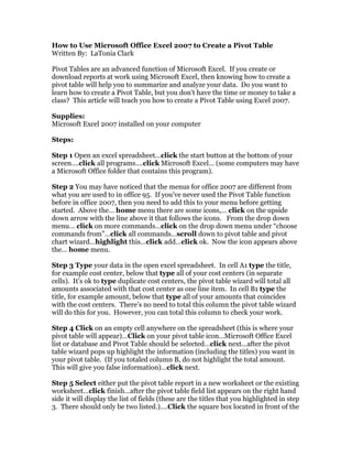
1. How to Use Microsoft Office Excel 2007 to Create a Pivot Table
Written By: LaTonia Clark
Pivot Tables are an advanced function of Microsoft Excel. If you create or
download reports at work using Microsoft Excel, then knowing how to create a
pivot table will help you to summarize and analyze your data. Do you want to
learn how to create a Pivot Table, but you don’t have the time or money to take a
class? This article will teach you how to create a Pivot Table using Excel 2007.
Supplies:
Microsoft Excel 2007 installed on your computer
Steps:
Step 1 Open an excel spreadsheet…click the start button at the bottom of your
screen….click all programs….click Microsoft Excel… (some computers may have
a Microsoft Office folder that contains this program).
Step 2 You may have noticed that the menus for office 2007 are different from
what you are used to in office 95. If you’ve never used the Pivot Table function
before in office 2007, then you need to add this to your menu before getting
started. Above the… home menu there are some icons,… click on the upside
down arrow with the line above it that follows the icons. From the drop down
menu… click on more commands…click on the drop down menu under “choose
commands from”…click all commands…scroll down to pivot table and pivot
chart wizard…highlight this…click add…click ok. Now the icon appears above
the… home menu.
Step 3 Type your data in the open excel spreadsheet. In cell A1 type the title,
for example cost center, below that type all of your cost centers (in separate
cells). It’s ok to type duplicate cost centers, the pivot table wizard will total all
amounts associated with that cost center as one line item. In cell B1 type the
title, for example amount, below that type all of your amounts that coincides
with the cost centers. There’s no need to total this column the pivot table wizard
will do this for you. However, you can total this column to check your work.
Step 4 Click on an empty cell anywhere on the spreadsheet (this is where your
pivot table will appear)…Click on your pivot table icon…Microsoft Office Excel
list or database and Pivot Table should be selected…click next…after the pivot
table wizard pops up highlight the information (including the titles) you want in
your pivot table. (If you totaled column B, do not highlight the total amount.
This will give you false information)…click next.
Step 5 Select either put the pivot table report in a new worksheet or the existing
worksheet…click finish…after the pivot table field list appears on the right hand
side it will display the list of fields (these are the titles that you highlighted in step
3. There should only be two listed.)….Click the square box located in front of the

2. fields (titles) you want to summarize in your pivot table, for example select cost
center and amount …click the “x” to close the pivot table field list.
Tips:
Tip 1 As a double check, check the total amount in column B against the grand
total in the pivot table you just created. If the amounts match that’s a good
indicator you performed this correctly.
Tip 2 Save your work.