The document discusses several key topics: 1) The First Fundamental Theorem of Calculus, which states that if f is continuous on [a,b] and F is an antiderivative of f, then the integral of f from a to x is equal to F(x) - F(a). 2) Examples of differentiating functions defined by integrals, including area functions and the error function (Erf). 3) The Second Fundamental Theorem of Calculus (weak form), which relates the integral of a continuous function f to antiderivatives F of f, stating that the integral of f from a to b is equal to F(b) - F(a).

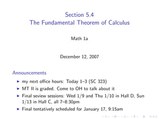
1. Section 5.4
The Fundamental Theorem of Calculus
Math 1a
December 12, 2007
Announcements
my next office hours: Today 1–3 (SC 323)
MT II is graded. Come to OH to talk about it
Final seview sessions: Wed 1/9 and Thu 1/10 in Hall D, Sun
1/13 in Hall C, all 7–8:30pm
Final tentatively scheduled for January 17, 9:15am

2. Outline
The Area Function
FTC1
Statement
Proof
Biographies
Differentiation of functions defined by integrals
“Contrived” examples
Erf
Other applications
FTC2
Facts about g from f
A problem

3. An area function
x
Let f (t) = t 2 and define g (x) = t 3 dt. Can we evaluate the
0
integral in g (x)?
x
0

4. An area function
x
Let f (t) = t 2 and define g (x) = t 3 dt. Can we evaluate the
0
integral in g (x)?
Dividing the interval [0, x] into n pieces
x ix
gives ∆x = and xi = 0 + i∆x = .
n n
So
x x 3 x (2x)3 x (nx)3
· 3+ · + ··· + ·
Rn =
n3 n3
nn n n
4
x
= 4 13 + 2 3 + 3 3 + · · · + n 3
n
x4 2
= 4 1 n(n + 1)
n2
x
0 x 4 n2 (n + 1)2 x4
→
=
4n4 4
as n → ∞.

5. An area function, continued
So
x4
g (x) = .
4

6. An area function, continued
So
x4
g (x) = .
4
This means that
g (x) = x 3 .

7. The area function
Let f be a function which is integrable (i.e., continuous or with
finitely many jump discontinuities) on [a, b]. Define
t
g (x) = f (t) dt.
a
When is g increasing?

8. The area function
Let f be a function which is integrable (i.e., continuous or with
finitely many jump discontinuities) on [a, b]. Define
t
g (x) = f (t) dt.
a
When is g increasing?
When is g decreasing?

9. The area function
Let f be a function which is integrable (i.e., continuous or with
finitely many jump discontinuities) on [a, b]. Define
t
g (x) = f (t) dt.
a
When is g increasing?
When is g decreasing?
Over a small interval, what’s the average rate of change of g ?

10. Outline
The Area Function
FTC1
Statement
Proof
Biographies
Differentiation of functions defined by integrals
“Contrived” examples
Erf
Other applications
FTC2
Facts about g from f
A problem

11. Theorem (The First Fundamental Theorem of Calculus)
Let f be an integrable function on [a, b] and define
x
g (x) = f (t) dt.
a
If f is continuous at x in (a, b), then g is differentiable at x and
g (x) = f (x).

12. Proof.
Let h > 0 be given so that x + h < b. We have
g (x + h) − g (x)
=
h

13. Proof.
Let h > 0 be given so that x + h < b. We have
x+h
g (x + h) − g (x) 1
= f (t) dt.
h h x

14. Proof.
Let h > 0 be given so that x + h < b. We have
x+h
g (x + h) − g (x) 1
= f (t) dt.
h h x
Let Mh be the maximum value of f on [x, x + h], and mh the
minimum value of f on [x, x + h]. From §5.2 we have
x+h
f (t) dt
x

15. Proof.
Let h > 0 be given so that x + h < b. We have
x+h
g (x + h) − g (x) 1
= f (t) dt.
h h x
Let Mh be the maximum value of f on [x, x + h], and mh the
minimum value of f on [x, x + h]. From §5.2 we have
x+h
f (t) dt ≤ Mh · h
x

16. Proof.
Let h > 0 be given so that x + h < b. We have
x+h
g (x + h) − g (x) 1
= f (t) dt.
h h x
Let Mh be the maximum value of f on [x, x + h], and mh the
minimum value of f on [x, x + h]. From §5.2 we have
x+h
mh · h ≤ f (t) dt ≤ Mh · h
x

17. Proof.
Let h > 0 be given so that x + h < b. We have
x+h
g (x + h) − g (x) 1
= f (t) dt.
h h x
Let Mh be the maximum value of f on [x, x + h], and mh the
minimum value of f on [x, x + h]. From §5.2 we have
x+h
mh · h ≤ f (t) dt ≤ Mh · h
x
So
g (x + h) − g (x)
mh ≤ ≤ Mh .
h

18. Proof.
Let h > 0 be given so that x + h < b. We have
x+h
g (x + h) − g (x) 1
= f (t) dt.
h h x
Let Mh be the maximum value of f on [x, x + h], and mh the
minimum value of f on [x, x + h]. From §5.2 we have
x+h
mh · h ≤ f (t) dt ≤ Mh · h
x
So
g (x + h) − g (x)
mh ≤ ≤ Mh .
h
As h → 0, both mh and Mh tend to f (x). Zappa-dappa.

19. Meet the Mathematician: Isaac Barrow
English, 1630-1677
Professor of Greek,
theology, and
mathematics at
Cambridge
Had a famous student

20. Meet the Mathematician: Isaac Newton
English, 1643–1727
Professor at Cambridge
(England)
Philosophiae Naturalis
Principia Mathematica
published 1687

21. Meet the Mathematician: Gottfried Leibniz
German, 1646–1716
Eminent philosopher as
well as mathematician
Contemporarily disgraced
by the calculus priority
dispute

22. Outline
The Area Function
FTC1
Statement
Proof
Biographies
Differentiation of functions defined by integrals
“Contrived” examples
Erf
Other applications
FTC2
Facts about g from f
A problem

23. Differentiation of area functions
Example
x
t 3 dt. We know g (x) = x 3 . What if instead we
Let g (x) =
0
had
3x
t 3 dt.
h(x) =
0
What is h (x)?

24. Differentiation of area functions
Example
x
t 3 dt. We know g (x) = x 3 . What if instead we
Let g (x) =
0
had
3x
t 3 dt.
h(x) =
0
What is h (x)?
Solution
We can think of h as the composition g ◦ k, where
u
t 3 dt and k(x) = 3x. Then
g (u) =
0
h (x) = g (k(x))k (x) = 3(k(x))3 = 3(3x)3 = 81x 3 .

25. Example
sin2 x
(17t 2 + 4t − 4) dt. What is h (x)?
Let h(x) =
0

26. Example
sin2 x
(17t 2 + 4t − 4) dt. What is h (x)?
Let h(x) =
0
Solution
We have
sin2 x
d
(17t 2 + 4t − 4) dt
dx 0
d
= 17(sin2 x)2 + 4(sin2 x) − 4 · sin2 x
dx
= 17 sin4 x + 4 sin2 x − 4 · 2 sin x cos x

27. Erf
Here’s a function with a funny name but an important role:
x
2 2
e −t dt.
erf(x) = √
π 0

28. Erf
Here’s a function with a funny name but an important role:
x
2 2
e −t dt.
erf(x) = √
π 0
It turns out erf is the shape of the bell curve.

29. Erf
Here’s a function with a funny name but an important role:
x
2 2
e −t dt.
erf(x) = √
π 0
It turns out erf is the shape of the bell curve. We can’t find erf(x),
explicitly, but we do know its derivative.
erf (x) =

30. Erf
Here’s a function with a funny name but an important role:
x
2 2
e −t dt.
erf(x) = √
π 0
It turns out erf is the shape of the bell curve. We can’t find erf(x),
explicitly, but we do know its derivative.
2 2
erf (x) = √ e −x .
π

31. Erf
Here’s a function with a funny name but an important role:
x
2 2
e −t dt.
erf(x) = √
π 0
It turns out erf is the shape of the bell curve. We can’t find erf(x),
explicitly, but we do know its derivative.
2 2
erf (x) = √ e −x .
π
Example
d
erf(x 2 ).
Find
dx

32. Erf
Here’s a function with a funny name but an important role:
x
2 2
e −t dt.
erf(x) = √
π 0
It turns out erf is the shape of the bell curve. We can’t find erf(x),
explicitly, but we do know its derivative.
2 2
erf (x) = √ e −x .
π
Example
d
erf(x 2 ).
Find
dx
Solution
By the chain rule we have
d d 2 4
22 4
erf(x 2 ) = erf (x 2 ) x 2 = √ e −(x ) 2x = √ xe −x .
dx dx π
2π

33. Other functions defined by integrals
The future value of an asset:
∞
π(τ )e −r τ dτ
FV (t) =
t
where π(τ ) is the profitability at time τ and r is the discount
rate.
The consumer surplus of a good:
p∗
CS(p ∗ ) = f (p) dp
0
where f (p) is the demand function and p ∗ is the equilibrium
price (depends on supply)

34. Outline
The Area Function
FTC1
Statement
Proof
Biographies
Differentiation of functions defined by integrals
“Contrived” examples
Erf
Other applications
FTC2
Facts about g from f
A problem

35. Theorem (The Second Fundamental Theorem of Calculus,
Weak Form)
If f is continuous on [a, b] and f = F for another function F , then
b
f (t) dt = F (b) − F (a).
a

36. Theorem (The Second Fundamental Theorem of Calculus,
Weak Form)
If f is continuous on [a, b] and f = F for another function F , then
b
f (t) dt = F (b) − F (a).
a
Proof.
Let g be the area function. Since f is continuous on [a, b], g is
differentiable on (a, b), and g = f = F on (a, b). Hence
g (x) = F (x) + C for all x in [a, b] (remember this requires the
Mean Value Theorem!). Since g (a) = 0, we have C = −F (a).
Therefore
g (b) = F (b) − F (a).

37. Outline
The Area Function
FTC1
Statement
Proof
Biographies
Differentiation of functions defined by integrals
“Contrived” examples
Erf
Other applications
FTC2
Facts about g from f
A problem

38. Facts about g from f
Let f be the function whose graph is given below.
Suppose the the position at time t seconds of a particle moving
t
along a coordinate axis is s(t) = f (x) dx meters. Use the
0
graph to answer the following questions.
4
3 •
(3,3)
2 • •
(2,2) (5,2)
1 •
(1,1)
1 2 3 4 5 6 7 8 9

39. Facts about g from f
Let f be the function whose graph is given below.
Suppose the the position at time t seconds of a particle moving
t
along a coordinate axis is s(t) = f (x) dx meters. Use the
0
graph to answer the following questions.
4
What is the particle’s velocity
3 •
(3,3) at time t = 5?
2 • •
(2,2) (5,2)
1 •
(1,1)
1 2 3 4 5 6 7 8 9

40. Facts about g from f
Let f be the function whose graph is given below.
Suppose the the position at time t seconds of a particle moving
t
along a coordinate axis is s(t) = f (x) dx meters. Use the
0
graph to answer the following questions.
4
What is the particle’s velocity
3 •
(3,3) at time t = 5?
2 • •
(2,2) (5,2) Solution
1 •
(1,1) Recall that by the FTC we
have
1 2 3 4 5 6 7 8 9
s (t) = f (t).
So s (5) = f (5) = 2.

41. Facts about g from f
Let f be the function whose graph is given below.
Suppose the the position at time t seconds of a particle moving
t
along a coordinate axis is s(t) = f (x) dx meters. Use the
0
graph to answer the following questions.
4
Is the acceleration of the par-
3 •
(3,3) ticle at time t = 5 positive or
2 negative?
• •
(2,2) (5,2)
1 •
(1,1)
1 2 3 4 5 6 7 8 9

42. Facts about g from f
Let f be the function whose graph is given below.
Suppose the the position at time t seconds of a particle moving
t
along a coordinate axis is s(t) = f (x) dx meters. Use the
0
graph to answer the following questions.
4
Is the acceleration of the par-
3 •
(3,3) ticle at time t = 5 positive or
2 negative?
• •
(2,2) (5,2)
1 •
(1,1) Solution
We have s (5) = f (5), which
1 2 3 4 5 6 7 8 9
looks negative from the
graph.

43. Facts about g from f
Let f be the function whose graph is given below.
Suppose the the position at time t seconds of a particle moving
t
along a coordinate axis is s(t) = f (x) dx meters. Use the
0
graph to answer the following questions.
4
What is the particle’s position
3 •
(3,3) at time t = 3?
2 • •
(2,2) (5,2)
1 •
(1,1)
1 2 3 4 5 6 7 8 9

44. Facts about g from f
Let f be the function whose graph is given below.
Suppose the the position at time t seconds of a particle moving
t
along a coordinate axis is s(t) = f (x) dx meters. Use the
0
graph to answer the following questions.
4
What is the particle’s position
3 •
(3,3) at time t = 3?
2 • •
(2,2) (5,2) Solution
1 •
(1,1) Since on [0, 3], f (x) = x, we
have
1 2 3 4 5 6 7 8 9
3
9
s(3) = x dx = .
2
0

45. Facts about g from f
Let f be the function whose graph is given below.
Suppose the the position at time t seconds of a particle moving
t
along a coordinate axis is s(t) = f (x) dx meters. Use the
0
graph to answer the following questions.
4
At what time during the first 9
3 •
(3,3) seconds does s have its largest
2 value?
• •
(2,2) (5,2)
1 •
(1,1)
1 2 3 4 5 6 7 8 9

46. Facts about g from f
Let f be the function whose graph is given below.
Suppose the the position at time t seconds of a particle moving
t
along a coordinate axis is s(t) = f (x) dx meters. Use the
0
graph to answer the following questions.
4
At what time during the first 9
3 •
(3,3) seconds does s have its largest
2 value?
• •
(2,2) (5,2)
1 •
(1,1) Solution
1 2 3 4 5 6 7 8 9

47. Facts about g from f
Let f be the function whose graph is given below.
Suppose the the position at time t seconds of a particle moving
t
along a coordinate axis is s(t) = f (x) dx meters. Use the
0
graph to answer the following questions.
4
At what time during the first 9
3 •
(3,3) seconds does s have its largest
2 value?
• •
(2,2) (5,2)
1 •
(1,1) Solution
The critical points of s are
1 2 3 4 5 6 7 8 9
the zeros of s = f .

48. Facts about g from f
Let f be the function whose graph is given below.
Suppose the the position at time t seconds of a particle moving
t
along a coordinate axis is s(t) = f (x) dx meters. Use the
0
graph to answer the following questions.
4
At what time during the first 9
3 •
(3,3) seconds does s have its largest
2 value?
• •
(2,2) (5,2)
1 •
(1,1) Solution
By looking at the graph, we
1 2 3 4 5 6 7 8 9
see that f is positive from
t = 0 to t = 6, then negative
from t = 6 to t = 9.

49. Facts about g from f
Let f be the function whose graph is given below.
Suppose the the position at time t seconds of a particle moving
t
along a coordinate axis is s(t) = f (x) dx meters. Use the
0
graph to answer the following questions.
4
At what time during the first 9
3 •
(3,3) seconds does s have its largest
2 value?
• •
(2,2) (5,2)
1 •
(1,1) Solution
Therefore s is increasing on
1 2 3 4 5 6 7 8 9
[0, 6], then decreasing on
[6, 9]. So its largest value is
at t = 6.

50. Facts about g from f
Let f be the function whose graph is given below.
Suppose the the position at time t seconds of a particle moving
t
along a coordinate axis is s(t) = f (x) dx meters. Use the
0
graph to answer the following questions.
4
Approximately when is the ac-
3 •
(3,3) celeration zero?
2 • •
(2,2) (5,2)
1 •
(1,1)
1 2 3 4 5 6 7 8 9

51. Facts about g from f
Let f be the function whose graph is given below.
Suppose the the position at time t seconds of a particle moving
t
along a coordinate axis is s(t) = f (x) dx meters. Use the
0
graph to answer the following questions.
4
Approximately when is the ac-
3 •
(3,3) celeration zero?
2 • •
(2,2) (5,2) Solution
1 •
(1,1) s = 0 when f = 0, which
happens at t = 4 and t = 7.5
1 2 3 4 5 6 7 8 9
(approximately)

52. Facts about g from f
Let f be the function whose graph is given below.
Suppose the the position at time t seconds of a particle moving
t
along a coordinate axis is s(t) = f (x) dx meters. Use the
0
graph to answer the following questions.
4
When is the particle moving
3 •
(3,3) toward the origin? Away from
2 the origin?
• •
(2,2) (5,2)
1 •
(1,1)
1 2 3 4 5 6 7 8 9

53. Facts about g from f
Let f be the function whose graph is given below.
Suppose the the position at time t seconds of a particle moving
t
along a coordinate axis is s(t) = f (x) dx meters. Use the
0
graph to answer the following questions.
4
When is the particle moving
3 •
(3,3) toward the origin? Away from
2 the origin?
• •
(2,2) (5,2)
1 •
(1,1) Solution
The particle is moving away
1 2 3 4 5 6 7 8 9
from the origin when s > 0
and s > 0.

54. Facts about g from f
Let f be the function whose graph is given below.
Suppose the the position at time t seconds of a particle moving
t
along a coordinate axis is s(t) = f (x) dx meters. Use the
0
graph to answer the following questions.
4
When is the particle moving
3 •
(3,3) toward the origin? Away from
2 the origin?
• •
(2,2) (5,2)
1 •
(1,1) Solution
Since s(0) = 0 and s > 0 on
1 2 3 4 5 6 7 8 9
(0, 6), we know the particle is
moving away from the origin
then.

55. Facts about g from f
Let f be the function whose graph is given below.
Suppose the the position at time t seconds of a particle moving
t
along a coordinate axis is s(t) = f (x) dx meters. Use the
0
graph to answer the following questions.
4
When is the particle moving
3 •
(3,3) toward the origin? Away from
2 the origin?
• •
(2,2) (5,2)
1 •
(1,1) Solution
After t = 6, s < 0, so the
1 2 3 4 5 6 7 8 9
particle is moving toward the
origin.

56. Facts about g from f
Let f be the function whose graph is given below.
Suppose the the position at time t seconds of a particle moving
t
along a coordinate axis is s(t) = f (x) dx meters. Use the
0
graph to answer the following questions.
4
On which side (positive or neg-
3 •
(3,3) ative) of the origin does the
2 • •
particle lie at time t = 9?
(2,2) (5,2)
1 •
(1,1)
1 2 3 4 5 6 7 8 9

57. Facts about g from f
Let f be the function whose graph is given below.
Suppose the the position at time t seconds of a particle moving
t
along a coordinate axis is s(t) = f (x) dx meters. Use the
0
graph to answer the following questions.
4
On which side (positive or neg-
3 •
(3,3) ative) of the origin does the
2 • •
particle lie at time t = 9?
(2,2) (5,2)
1 •
(1,1) Solution
We have s(9) =
1 2 3 4 5 6 7 8 9 6 9
f (x) dx + f (x) dx,
0 6
where the left integral is
positive and the right integral
is negative.

58. Facts about g from f
Let f be the function whose graph is given below.
Suppose the the position at time t seconds of a particle moving
t
along a coordinate axis is s(t) = f (x) dx meters. Use the
0
graph to answer the following questions.
4
On which side (positive or neg-
3 •
(3,3) ative) of the origin does the
2 • •
particle lie at time t = 9?
(2,2) (5,2)
1 •
(1,1) Solution
In order to decide whether
1 2 3 4 5 6 7 8 9
s(9) is positive or negative,
we need to decide if the first
area is more positive than the
second area is negative.

59. Facts about g from f
Let f be the function whose graph is given below.
Suppose the the position at time t seconds of a particle moving
t
along a coordinate axis is s(t) = f (x) dx meters. Use the
0
graph to answer the following questions.
4
On which side (positive or neg-
3 •
(3,3) ative) of the origin does the
2 • •
particle lie at time t = 9?
(2,2) (5,2)
1 •
(1,1) Solution
This appears to be the case,
1 2 3 4 5 6 7 8 9
so s(9) is positive.