The Latin square design is used where the researcher desires to control the variation in an experiment that is related to rows and columns in the field.

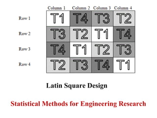
1. Statistical Methods for Engineering Research
Latin Square Design

2. Prepared By
Dr. Manu Melwin Joy
Assistant Professor
School of Management Studies
Cochin University of Science and Technology
Kerala, India.
Phone – 9744551114
Mail – manumelwinjoy@cusat.ac.in
Kindly restrict the use of slides for personal purpose.
Please seek permission to reproduce the same in public forms and
presentations.

3. Latin Square Design
• The Latin square design is used where the
researcher desires to control the variation in an
experiment that is related to rows and columns
in the field.

4. Definition
• A Latin square is a square array of objects (letters A,
B, C, …) such that each object appears once and only
once in each row and each column. Example - 4 x 4
Latin Square.
A B C D
B C D A
C D A B
D A B C

5. In a Latin square You have three factors:
• Treatments (t) (letters A, B, C, …)
• Rows (t)
• Columns (t)
The number of treatments = the number of rows =
the number of colums = t.
The row-column treatments are represented by cells
in a t x t array.
The treatments are assigned to row-column
combinations using a Latin-square arrangement

6. Example
A courier company is interested in deciding
between five brands (D,P,F,C and R) of car
for its next purchase of fleet cars.
• The brands are all comparable in purchase price.
• The company wants to carry out a study that will
enable them to compare the brands with respect to
operating costs.
• For this purpose they select five drivers (Rows).
• In addition the study will be carried out over a
five week period (Columns = weeks).

7. • Each week a driver is assigned to a car using
randomization and a Latin Square Design.
• The average cost per mile is recorded at the end of
each week and is tabulated below:
Week
1 2 3 4 5
1 5.83 6.22 7.67 9.43 6.57
D P F C R
2 4.80 7.56 10.34 5.82 9.86
P D C R F
Drivers 3 7.43 11.29 7.01 10.48 9.27
F C R D P
4 6.60 9.54 11.11 10.84 15.05
R F D P C
5 11.24 6.34 11.30 12.58 16.04
C R P F D

8. The Model for a Latin Experiment
( ) ( )kijjikkijy εγρτµ ++++=
i = 1,2,…, t j = 1,2,…, t
yij(k) = the observation in ith
row and the jth
column receiving the kth
treatment
µ = overall mean
τk = the effect of the ith
treatment
ρi = the effect of the ith
row
εij(k) = random error
k = 1,2,…, t
γj = the effect of the jth
column
No interaction
between rows,
columns and
treatments

9. • A Latin Square experiment is assumed to be a
three-factor experiment.
• The factors are rows, columns and treatments.
• It is assumed that there is no interaction between
rows, columns and treatments.
• The degrees of freedom for the interactions is
used to estimate error.

10. Example 2
In this Experiment the we are again interested in how
weight gain (Y) in rats is affected by Source of
protein (Beef, Cereal, and Pork) and by Level of
Protein (High or Low).
There are a total of t = 3 X 2 = 6 treatment
combinations of the two factors.
• Beef -High Protein
• Cereal-High Protein
• Pork-High Protein
• Beef -Low Protein
• Cereal-Low Protein and
• Pork-Low Protein

11. In this example we will consider using a Latin Square
design
Six Initial Weight categories are identified for the
test animals in addition to Six Appetite categories.
• A test animal is then selected from each of the 6 X
6 = 36 combinations of Initial Weight and
Appetite categories.
• A Latin square is then used to assign the 6 diets to
the 36 test animals in the study.

12. In the latin square the letter
• A represents the high protein-cereal diet
• B represents the high protein-pork diet
• C represents the low protein-beef Diet
• D represents the low protein-cereal diet
• E represents the low protein-pork diet and
• F represents the high protein-beef diet.

13. The weight gain after a fixed period is measured for
each of the test animals and is tabulated below:
Appetite Category
1 2 3 4 5 6
1 62.1 84.3 61.5 66.3 73.0 104.7
A B C D E F
2 86.2 91.9 69.2 64.5 80.8 83.9
B F D C A E
Initial 3 63.9 71.1 69.6 90.4 100.7 93.2
Weight C D E F B A
Category 4 68.9 77.2 97.3 72.1 81.7 114.7
D A F E C B
5 73.8 73.3 78.6 101.9 111.5 95.3
E C A B F D
6 101.8 83.8 110.6 87.9 93.5 103.8
F E B A D C