Simple and Collaborative Slideshow for Working with Dropdown lists in Excel 2013 If the video does not work,Please download and check (Sorry if the inconvenience is caused) Hope you like it, Free to download and share, Check our Other Tutorials onto other Microsoft Office Softwares and further more into miscellaneous slideshows.

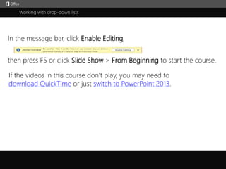
1. Working with drop-down lists
j
then press F5 or click Slide Show > From Beginning to start the course.
In the message bar, click Enable Editing,
If the videos in this course don’t play, you may need to
download QuickTime or just switch to PowerPoint 2013.

2. 5 761 2 3 4
Course summary Help
Press F5 to start, Esc to stop 1/4 videos
Working with drop-down lists Closed captions
Summary Feedback HelpDrop-down lists Settings Messages Manage lists
2:47 6:201:01 4:37
Data entry is quicker and more accurate when you use a drop-down listto limit the entries people can make in a cell.When you select a cell, the drop-down list’s down-arrow appears.Click it and make a selection.Here’s how to create drop-down lists:Select the cells that you want to contain the lists.On the ribbon, click the Data tab, and click Data Validation.In the dialog, set Allow to List.Click in Source.In this example, we’re using a comma-delimited list.The text or numbers we type in the Source field are separated by commas.And click OK.The cells now have a drop-down lists.Up next, drop-down list settings.

3. 5 761 2 3 4
Course summary Help
Press F5 to start, Esc to stop 2/4 videos
Working with drop-down lists Closed captions
Summary Feedback HelpDrop-down lists Settings Messages Manage lists
2:47 6:201:01 4:37
You can use a comma-delimited list, a cell range, or a named range to define the options in a drop-down
list.
We used a comma-delimited list in the previous video.You might use such a list if there are just a few values and they’re unlikely to change.If you need to change the list entries, such as adding and deleting entries,this type of drop-down list is more time-consuming to manage.We’ll cover managing drop-down lists in video 4.A comma-delimited list is also case sensitive.This can be a problem when someone types an entry instead of picking it from the list.For example, typing YES in all capital letters returns an error, if error messages are enabled, which is the
default.
To avoid the problem, let’s use a cell range for the entries in the drop-down list.Select a cell where you want a drop-down list.Click the Data tab, and click Data Validation.In the Data Validation dialog, set Allow to List; this enables a list in the cell.Leave In-cell dropdown selected; this enables a drop-down list in the cell.Leave Ignore blank selected; we’ll cover this in the next video.To provide the options in your drop-down list, click in Source and select the cell range that contains those
options.
• It can be on a different worksheet, as in this example,giving you greater flexibility in configuring and protecting the worksheets. We’ll cover this in video 4.• The range must be a single row or column.And click OK.Verify the cell contains a drop-down list with the options provided by the cell range.To use this drop-down list in other locations, copy it to other cells.Select the cell.If it shows a text or number entry, press Delete to clear it.This way, text and numbers won’t appear in the destination cells, so it doesn’t seem like an entry was already
selected.
You can use the keyboard shortcut Ctrl + C to copy the cell.Then select the destination cellsAnd press Ctrl + V to paste it.These cells now have the drop-down list.A named range, such as Fruits, is easier to remember than a cell range, such as A2:A37.To use a named range for the options in your drop-down list, you start by creating one.Select the cell range you want to name.In the Name Box, type the name you want for the range. For example, underscore Veggies.• The first character of a name must be a letter or an underscore.• The rest of the name can be letters, numbers, periods, and underscores.• A name can’t have spaces.• And you can’t use Predefined statements, such as true or false, or cell references, such as A1.When you select the cells of a named range, you’ll see the name in the Name Box.Now you’re ready to create a drop-down list that uses the named range.Select a cell where you want a drop-down list.Click Data Validation.Select List.Click in Source, press F3, select the name, and click OK, and click OK again.Verify that the cell contains the drop-down list with the entries provided by the named range.And copy the list to other cells.Up next, input and error messages.

4. 5 761 2 3 4
Course summary Help
Press F5 to start, Esc to stop 3/4 videos
Working with drop-down lists Closed captions
Summary Feedback HelpDrop-down lists Settings Messages Manage lists
2:47 6:201:01 4:37
To help people decide what drop-down list option to select, and even to let them know that a cell contains a
drop-down list,
you can create a message that appears when they select a cell.You can add the message to all cells that contain the drop-down list, or just the first cell in a column.Select the cells that you want to create a message for, and click Data Validation.On the Input Message tab, check the box next to Show input message when cell is selected.Type a title if you want. It’ll appear in bold.Type the message in the Input message box.Now when you click a cell, the message pops up.You can let people type blank entries in cells that have a drop-down list.If Ignore blank is checked in the Data Validation dialog, which it is by default, people can enter blanks.If you uncheck Ignore blank and someone enters a blank entry,an error message shows if Error Alert is enabled for the drop-down list, as it is by default.We’ll go over error messages next.By default, someone can select or type only values that are in the drop-down list.If they type a different value, they get an error message and can’t enter the value if the default error style,called Stop, is enabled for the drop-down list.You can provide your own error message and also allow people to type their own values. Here’s how:Select the cells you want.Click Data Validation.Click the Error Alert tab and check the box.The default error style is Stop. As we’ve seen, this prevents people from entering values that aren’t in the
drop-down list.
Type a title if you want, and type the error message.When people type a value that isn’t in the drop-down list, they now see your customized error message.The Warning and Information error messages allow people to enter a value that isn’t in the drop-down list.If you don’t want an error message, clear the check box.Up Next: Manage drop-down lists.

5. 5 761 2 3 4
Course summary Help
Press F5 to start, Esc to stop 4/4 videos
Working with drop-down lists Closed captions
Summary Feedback HelpDrop-down lists Settings Messages Manage lists
2:47 6:201:01 4:37
To prevent anyone from accidentally changing the drop-down list data,you can hide the columns, rows, or the entire worksheet that contains the data.You can then unhide them if you need to make changes.You can also lock and password protect the cells on the worksheet or even the entire worksheet.By password protecting the data, only people with the password can make changes.But it’ll also require a little more effort on your part if you decide to make changes,because you have to unprotect the data first.To hide columns or rows, select the columns or rows, right-click them, and click Hide.To unhide them, select the column or row on one side of the hidden columns or rows, drag your mouse to
the other side,
right-click, and click Unhide.To hide a worksheet, right-click the worksheet’s tab, and click Hide.To unhide a worksheet, right-click any worksheet tab, click Unhide, and click OK.By default, all cells on a worksheet are locked. But this has no effect until the worksheet is password
protected.
To password protect a worksheet, right-click its tab and click Protect Sheet.Enter the password and click OK.Reenter the password and click OK again.Now if I try to type in any cell on the worksheet, I get an error.To unprotect a worksheet, right-click the worksheet’s tab, click Unprotect Sheet, enter the password, and
click OK.
To lock specific cells, you first have to change the default for the worksheet.Select the entire worksheet, right-click it, and click Format Cells.In Format Cells, click the Protection tab, uncheck Locked, and click OK.Select the specific cells you want to lock, right-click them, and click Format Cells.In Format Cells, check Locked, and click OK.Then password protect the worksheet.Only these cells on the worksheet are locked.I can type in an unlocked cell, but if I try to type in a locked cell I get an error.To change the options for a drop-down list you edit the data for the drop-down listand the possibly the data validation Source field.For a drop-down list that uses a comma-delimited list in the Source field, select the cells with the drop-down
list,
and in the data validation Source field make the desired changes to the comma-delimited list.And click OK.And we can see the updated list options.For a drop-down list that’s based on a cell range, click a cell in the range and type the changes you want to
make.
To insert a drop-down list option, right-click a cell in the range, click Insert, click OK,and type your new option in the cell. Deleting a cell works similarly.And again, we can see the updated list options.You can also select the cells in the drop-down list, click Data Validation, and set Source to the new cell
range.
For a drop-down list that’s based on a named range, click a cell in the range and type the change you want
to make.
To insert a drop-down list option, right-click a cell in the range,click Insert, click OK, and type your new option in the cell. Deleting a cell works similarly.And again, we can see the updated list options.To edit or delete a named range, click the Formulas tab, and click Name Manager.In Name Manager, select the desired name, and click Edit or Delete.To delete a drop-down list from cells, select the cells, click Data Validation, click Clear All, and click OK.The drop-down list is removed from the cells, but not the values that have been selected.You can remove those by pressing Delete.Now you’ve got a pretty good idea about how to apply and use drop-down lists in Excel.Of course, there’s always more to learn.So check out the course summary at the end, and best of all, explore Excel 2013 on your own.

6. Help Course summary
Press F5 to start, Esc to stop
Course summary—Working with drop-down lists
Summary Feedback Help
5 761 2 3 4
Drop-down lists Settings Messages Manage lists
2:47 6:201:01 4:37
Create a drop-down list
You can make a worksheet more efficient by providing
drop-down lists. Someone using your worksheet clicks
an arrow, and then clicks an entry in the list.
1. Select the cells that you want to contain the lists.
2. On the ribbon, click Data > Data Validation.
3. In the dialog, set Allow to List.
4. Click in Source, type the text or numbers
(separated by commas, for a comma-delimited list)
you want in your drop down list, and click OK.
Lock cells to protect them
Your boss wanted you to protect a workbook, but she
also wanted to be able to change a few cells after you
were done. So, you unlocked some cells. Now your
boss is done, so you can lock the cells. Here's how.
1. Select the cells you want to lock.
2. Click Home, then click the Format Cell dialog box
launcher (the arrow to the right of Alignment in
the ribbon).
3. Click the Protection tab, check the Locked box,
and click OK.
4. Click Review > Protect Sheet or Protect
Workbook and reapply protection.
Create input and error messages
To help people decide what drop-down list option to
select, and even to let them know that a cell contains a
drop-down list, you can create a message that appears
when they select a cell. You can add the message to all
cells that contain the drop-down list, or just the first cell
in a column.
1. Select the cells that you want to create a message
for, and click Data Validation.
2. On the Input Message tab, check the box next to
Show input message when cell is selected.
3. Type a title if you want. It’ll appear in bold.
4. Type the message in the Input message box. Now
when you click a cell, the message pops up.
See also
• More training courses
• Office Compatibility Pack
• Create a drop-down list
• Add or remove items from a drop-down
list
• Remove a drop-down list
• Lock cells to protect them

7. Check out more courses
Help Course summary
Press F5 to start, Esc to stop
Rating and comments
Thank you for viewing this course!
Please tell us what you think
Summary Feedback Help
5 761 2 3 4
Drop-down lists Settings Messages Manage lists
2:47 6:201:01 4:37

8. Help Course summary
Press F5 to start, Esc to stop
Help
Summary Feedback Help
5 761 2 3 4
Using PowerPoint’s video controls
Going places
Stopping a course
If you download a course and the videos don’t play
get the PowerPoint Viewer. the QuickTime
player upgrade to PowerPoint 2013
Drop-down lists Settings Messages Manage lists
2:47 6:201:01 4:37