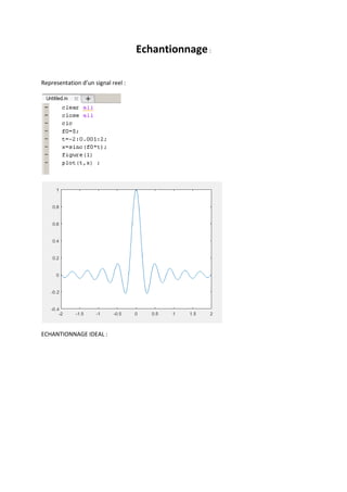
1) The document discusses signal sampling and representation of real signals.
2) It presents ideal sampling and shows the effect of varying sampling rates on a sinc signal.
3) It applies an averaging function to downsample sinc signals sampled at different rates, and plots the results.
7. clear all
close all
clc
f0=5;
t=-2:0.001:2;
x=sinc(f0*t);
figure(1)
plot(t,x) ;
fe1=5;
Te1=1/fe1;
t1=-2:Te1:2;
x1=sinc(f0*t1);
fe2=10;
Te2=1/fe2;
t2=-2:Te2:2;
x2=sinc(f0*t2);
figure(2)
fe3=30;
Te3=1/fe3;
t3=-2:Te3:2;
x3=sinc(f0*t3);
hold on
plot(t1,x1,'b');
plot(t2,x2,'r');
plot(t3,x3,'G');
hold off
deltat1=Te1;
moy1=moyenneur(x,t,Te1,deltat1);
figure(3)
hold on
plot(t,x,'r');
8. plot(t1,moy1);
hold off
deltat2=Te1/5;
moy2=moyenneur(x,t,Te1,deltat2);
figure(4)
hold on
plot(t,x)
plot(t1,moy2,'b');
hold off
moy3=moyenneur(x,t,Te2,deltat1);
figure(5)
hold on
plot(t,x)
plot(t2,moy3,'b')
hold off
moy4=moyenneur(x,t,Te2,deltat2);
figure(6)
hold on
plot(t2,moy4);
plot(t,x);
hold off
moy5=moyenneur(x,t,Te3,deltat1);
figure(7)
hold on
plot(t3,moy5);
plot(t,x);
hold off
moy6=moyenneur(x,t,Te3,deltat2);
figure(8)
hold on
plot(t3,moy6);
plot(t,x);
hold off
function moy=moyenneur(x,t,Te,deltaT);
tech=-2:Te:2;
for n=1:length(tech)
nb_points=find((t>=tech(n))&(t<tech(n)+deltaT));
Xech_reel(n)=mean(x(nb_points));
end
moy=Xech_reel;
end