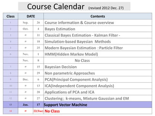
1. Course Calendar (revised 2012 Dec. 27)
Class DATE Contents
1 Sep. 26 Course information & Course overview
2 Oct. 4 Bayes Estimation
3 〃 11 Classical Bayes Estimation - Kalman Filter -
4 〃 18 Simulation-based Bayesian Methods
5 〃 25 Modern Bayesian Estimation ：Particle Filter
6 Nov. 1 HMM(Hidden Markov Model)
Nov. 8 No Class
7 〃 15 Bayesian Decision
8 〃 29 Non parametric Approaches
9 Dec. 6 PCA(Principal Component Analysis)
10 〃 13 ICA(Independent Component Analysis)
11 〃 20 Applications of PCA and ICA
12 〃 27 Clustering； k-means, Mixture Gaussian and EM
13 Jan. 17 Support Vector Machine
14 〃 22(Tue) No Class

2. Lecture Plan
Support Vector Machine
1. Linear Discriminative Machine
Perceptron Learning rule
2. Support Vector Machine
Problem setting, Optimization
3. Generalization of SVM

3. 3
１. Introduction
1.1 Classical Linear Discriminative Function
-Perceptron Machine-
Consider the two-category linear discriminative problem using
perceptron-type machine.
- Assumption
Two-category (𝐶1 , 𝐶2) training data in D-dimensional feature space are
separable by a linear discriminative function of the form
𝑓 𝑥 = 𝑤 𝑇 𝑥
which satisfies
𝑓 𝑥 ≥ 0 𝑓𝑜𝑟 𝑥 ∈ 𝐶1
𝑓 𝑥 < 0 𝑓𝑜𝑟 𝑥 ∈ 𝐶2
 
 
 
0 1
0 1
where , , , is (D+1)-dim. weight vector
1, , ,
Here, 0 gives the hyperplane surface which separates
two categories and its normal vector is .
T
D
T
D
T
w w w w
x x x x
f x w x
w

 
 

4. 4
𝑤0
𝑥0 = 1
+
𝑤1
𝑥1
𝑤 𝐷𝑥 𝐷
.
.
.
.
 
0
D
i i
i
f x w x

 
Fig. 1 Perceptron
Class C1
Class C2
Hyperplane f(x)=0
Fig. 2 Linear Discrimination
weights
x-space

5. 5
( )
2
( ) ( ) ( ) ( )
2
(0)
(1) (2)
( 1) ( )
- Reverse the training vectors of class C
for
- Initial weight vector :
- For a new training dataset , , ,
if
i
i new i i i
i i
x
x x x x C
w
x x
w w
   
  
 
( )
( 1) ( ) ( ) ( )
0
+ if 0
where determines the convergence speed of learning.
i
i i i i
f x
w w x f x



 
1.2 Learning Rule of Perceptron (η=1 case)
Class C1
Reversed C2 data
Fig. 3 Reversed data of class C2
reflect

6. 6
Training data
H0
w0
H1
x1
＋
－
H0
w0
x1
＋－
w1
=w0+x1
(a) i=0
(b) i=1
Illustration of weight
update scheme

7. 7
H1
H2
w0
x1
＋
－
w1
=w0+x1
x2 H0
w2=w1+x2
(c) i=2
Fig. 4 Learning process of Perceptron

8. 8
2. Support Vector Machine (SVM)
2.1 Problem Setting
Given a linearly separable two-category(𝐶1 , 𝐶2) training dataset with
class labels
𝑥𝑖, 𝑡𝑖 𝑖 = 1~𝑁
where 𝑥𝑖 ∶ D-dimensional feature vector
𝑡𝑖 = {−1,1} “1” for C1, and “ -1” for C2
Find a separating hyperplane H
𝑓 𝑥 = 𝑤 𝑇 𝑥 + 𝑏 = 0
- Among a set of possible hyperplanes, we want to seek a reasonable
hyperplane which is farthest from all training sample vectors.
- The obtained discriminant hyperplane will give better generalization
capability. (*)
(*) It is expected well for test data which are outside the training data

9. 9
Motivation of SVM
The optimal discriminative hyperplane should have the largest
margin which is defined as the minimum distance of the training
vectors to the separation surface.
Class C1
Class C2
Margin
Fig. 5 Margin
Hyperplane

10. 10
The distance between a hyperplane
0
and a sample point is given by
(see Appendix)
Since both the scalar( )-multiplication ( ) and a pair
T
i
T
i
w x b
x
w x b
w
k kw,kb
 

2.2 Optimization problem
of ( , )
give the same hyperplane, we choose the optimal hyperplane which
is given by the discriminative function
1
where in (3) is the closest vector to the separation surface.
T
i
i
w b
w x b
x
 
(Canonical hyperplane)
(1)
(2)
(3)

11. 11
2
2
0
p
T T
p
b
x w w
w
w x b w w b
b
w




 
     
 
   
 
ix
qx

px
w
w
hyperplane
0T
w x b 
2
2
= ( = )
T T
i i
q q q
TT
ii
q p
w x w xw
x x w x
w ww
w x bw x b
x x w
ww
 


    
:distance between
and hyperplane
ix

Appendix
Fig.6

12. 12
1
2
- The distance (2) from the closest training vector to the decision
surface is
1
2
- The margin is
- If 1 (C ) then 1
If 1 (C ) then 1
therefore
T
i
T
i i
T
i i
w x b
w w
w
t w x b
t w x b


  
   
  1T
i it w x b 
Fig. ７ Margin and distance
Hyperplane
T
iw x b
w

2
w
(4)
(5)

13. 13
 
2
- Maximization of the margin-
1 1
Minimize
2 2
Subject to ( ) 1 ( 1~ )
Since ( ) is a quadratic function with respect to , there exists
T
T
i i
J w w w w
t w x b i N
J w w
 
  
Optimization problem
an (unique) global minimum.
(7)
(6)

14. 14
 
 
* *
*
*
satisfies
( , )
(i) 0
(ii) 0 ( 1,..., )
(iii) 0
(iv) 0
z z
i i
i
i
L z
z
g z i k
g z








 


 
(optimiztion conditions)
Minimize z (convex space)
Subject to ( ) 0 ( 1~ )
The necessary and suffi
i
J z
g z i k

 
2.3 Lagrangian multiplier approach - general theory -
Kuhn - Tucker Theorem
 
*
*
1
cient conditions for a point to be
an optimum are the existence of such that the Lagrangian function
( , ): ( )
k
i i
i
z
L z J z g z

 

   (8)
(9)
(10)
(11)
(12)

15. 15
- The second condition (10), called Karush-Kuhn-Tucker(KKT)
condition or complementary condition, implies the following facts
ifor active constraints if α >0
and for inactive constr iaints if α = 0
 
 
1
Apply K-T theorem to Eq. (6) (7)
- Lagrangian
1
( , , ): 1
2
- Condition (i) by substituting , gives
( , , )
0
T T
p i i i
N
p
i i i
i
L w b w w t w x b
z w b
L w b
w t x
w
 



     


  



2.4 Dual Problem
1
( , , )
0 0
N
p
i i
i
L w b
t
b




  


(13)
(14)
(15)

16. 16
 
0
1
1 1 1
1
1
( , , )
2
1 1
2 2
1 1
2 2
1
2
1
(: ( , , )) =
2
T T
p i i i i i i
i i i
I
K
N
T T
i i i
i
N N N
T T
i i i i i i i i i
i i i
N
T
i j i j i j
i j
p i
i
L w b w w t w x b t
I w w w t x
K t w x t t x x
t t x x
L L w b
   

  
 
  


  

   
 
 
     
 
 
  
  

  

 1
1
is maximized subject to
0 and 0
N
T
i j i j i j
i j
N
i i i
i
t t x x
t
 
 


 


(16)
(17)

17. 17
 
 
 
- Dual problem is easier to solve because depends only
on not on ,
- contains training data as the inner product form
- Geometric interpretation of KKT condition (ii) or Eq.(10)
i
T
i i j
L
w b
L x x x



 
 
1 0 1
mans,
at either =0 or 1 must hold.
for some 0 must lie on one of the hyperplanes
,namely with active constraint provides the largest margin.
T
i i i
T
i i i i
j
j
t w x b i N
x t w x b
x



     
 

(Such is called support vector, see Fig. 8)
At all other points 0 (inactive constraint points)
j
i
x
 
(18)

18. 18
0
- Only the support vectors contribute to determine hyperplane
because of
- The KTT condition is used to determine the bias b.
i
i i i i iw t x t x



  
Fig. 8 KTT conditions
support vectors
𝛼𝑖 > 0
𝛼𝑖 = 0
𝛼𝑖 = 0
inactive constraint points
0
- Hyperplane : 0
i
T
i it x x b
 
 
(19)
(20)

19. 19
3. Generalization of SVM
3 .1 Non-separable case
- Introduce slack variables ξi in order to relax the constraint (7) as
follows;
𝑡𝑖(𝑤 𝑇 𝑥𝑖 + 𝑏) ≥1－ ξi
For ξi =0, the data point is correctly separable with margin.
For 0≦ξi ≦1, the data point is separable but falls within the region of
the margin.
For ξi >1, the data point falls on the wrong side of the separating surface.
Define the slack variable
ξi := ramp{1－𝑡𝑖(𝑤 𝑇 𝑥𝑖 + 𝑏)}
where ramp{u} = u for u>0 and =0 for u≦0.
 
 
1
New Optimization Problem:
1
Minimize , :=
2
subject to 1+ 0
0 ( 1 )
N
T
p i
i
T
i i i
L w w w C
t w x b
i N
 




  
 

(21)
(22)

20. 20
Fig. 9 Non separable case and stack variable
𝑡𝑖 = 1
𝑡𝑖 = −1
 0
0 0
0
1T
w x b
 
 
 0
0
0.5
1
2
T
w x b
 
 
 0
0 0
1.5
1
2
T
w x b
 
  
 00 0 1
optimum hyperplane
0T
w x b   
support vectors
i

21. 21
3.2 Nonlinear SVM
- For the separation problem by a nonlinear discriminative surface,
nonlinear mapping approach is useful.
- Cover’s theorem: A complex pattern classification problem cast in a
high-dimensional space non-linearly is more likely to be linearly
separable than in a low-dimensional space.
x ( )x ( )z x SVM
higher dimension
Fig. 10 nonlinear mapping
( )z x
x-space z-space

22. 22
       
   
 
   
0 1
0
1, , , ( )
- Hyperplane in -space: 0
- SVM in -space gives an optimum hyperplane with the form
(sum of support vectors in )
- Discriminat
T
M
T
i i i i
i
x x x x M D
x w x
x
w t x x
   
 

  
    

 
     
 
     
0
inner product
in M-d space
inner product in -domain kernel function in -domain
ive function:
- If we can choose which satisfies
,
the co
T T
i i i
i
T
i j i j
x
w x t x x
x
x x K x x

   

 



mputational cost will be drastically reduced.
(23)
(24)
(25)

23. 23
       
 
2
2 2
1 1 2 2 1 2
) Polynomial kernel
, 1
where 1, , 2 , , 2 , 2
T T
T
Ex
K u v u v u v
v u u u u u u
 

  
   
Ex) Nonlinear SVM result by utilizing Gauss kernel
Fig. 11
Support vectors
Bishop [1]

24. 24
References:
[1] C. M. Bishop, “Pattern Recognition and Machine Learning”,
Springer, 2006
[2] R.O. Duda, P.E. Hart, and D. G. Stork, “Pattern Classification”,
John Wiley & Sons, 2nd edition, 2004
[3] 平井有三 「はじめてのパターン認識」森北出版(2012年)