SlideShare a Scribd company logo
1 of 82
Electric Circuits Lab
Inductors in DC Circuits
I.
Objectives:
After completing this lab experiment, you should be able to:
· Measure the resistance and Inductance.
· Use the Oscilloscope and Function generator.
· Measure the LR time constant using VR and VL.
· Understand the effect of series and parallel inductors on LR
time constant.
II.
Parts List:
· Resistor (1) 5.1 kΩ
· Inductor (2) 100mH
III.
Procedures:
Part I:
1.
Construct the circuit shown in
Figure 1 in Multisim. (You may use either the clock
voltage component or the function generator.)
PP
Figure 1: RL Circuit
2.
Connect Channel A of the oscilloscope across the
resistor and Channel B across the inductor.
3.
Set the voltage source to
5VPP; 300 Hz, Square wave, 50% duty cycle
4. You should be able to see the waveform as shown below.
(Use Volts/Div and Time/DIV settings to adjust the signal)
Figure 2. Voltage across the inductor and resistor
5.
Calculate the time constant of an LR circuit.
Record the result in
Table 1 below under the calculated value.
Calculated value
Measured value using VL
Measured value using VR
19.6 us
20.319 us
20.398 us
Table 1: Calculated and measured time constant values
6. Turn on the cursors on the oscilloscope
7.
Measuring the time constant with VL: (shown in Figure
3)
i.
Set Channel A to “0” to turn off Channel A signal.
ii.
Measure the peak value of the voltage across the
resistor, by placing one of the cursors at the peak point
_____5.002 V____.
iii.
Calculate the 37% of the above value ___1.85V______.
iv.
Place the second cursor at the voltage calculated above
in step (iii).
v.
Observe the change in time (T2-T1) value on the scope,
which is the value of one time constant.
vi.
Record the T2-T1 value in
Table 1 above under measured value using VL.
Figure 3: Measuring RL time constant using VL example (L =
150 mH)
Note: your scope screen will be different
8.
Set Channel B to “0” to turn it off.
9.
Set Channel A to “AC”
10. Adjust the Trigger settings, if needed, and you should be
able to see the waveform as shown below. (Use Volts/Div and
Time/DIV knobs to adjust the signal)
Figure 4: Voltage across the resistor
11.
Measuring the time constant: (shown in Figure 5)
i.
Measure the peak value of the signal, by placing one of
the cursors (T1) at the peak point and the other cursor (T2) at
the negative peak.
Calculate the total peak-to-peak voltage (T1-T2)
_4.998V________.
ii.
Calculate the 63% of the above value __3.15V_______.
iii.
Place the second cursor (T2) at the negative peak value
plus the step (ii) value above
.
iv.
Place T1 at the negative peak just before the signal
begins to rise.
vii.
Observe the dT (T2-T1) value on the scope, which is
one time constant.
viii.
Record the result in
Table 1 above under measured value using VR.
Figure 5: Measuring RL time constant using VR example (L =
150 mH)
Note: your scope screen will be different
Part II:
12.
Place two inductors in series as shown below.
Figure 6: Series Inductors
13.
Calculate the total inductance value and
record the results in
Table 2 (Calculated) below.
14.
Measure the total inductance value. (If you have the
proper measuring device to do so). Use the following procedure
to measure the inductance in Multisim if you do not have the
proper measuring device.
i.
Connect the Impedance Meter (Simulate
>>Instruments>>LabView Instruments>>Impedance Meter) as
shown in
Figure 7.
ii.
Measure the inductive reactance, XL, as shown in
Figure 7
.
iii.
Calculate the inductance using the equation. and
record the value in
Table 2 (Measured).
Calculated Value
Measured Value
Inductance
200
199.99
Table 2: Series Inductors
Figure 7. Impedance Meter in Multisim Example
15.
Build the circuit in
Figure 8.
Figure 8: RL circuit with series Inductors
16.
Calculate the new LR time constant.
Record the result in
Table 3 below.
17.
Connect Channel A of the oscilloscope across the
resistor.
18. Adjust the Trigger, if needed, and you should be able to see
the waveform as shown below. (Use Volts/Div and Time/DIV
knobs to adjust the signal)
Figure 9: Voltage across the resistor
19. Use the cursors on the oscilloscope to
measure the time constant (refer to step 11).
Record the result in
Table 3 below under measured value.
Calculated value
Measured value using VR
40 us
41.276 us
Table 3: Calculated and measured time constant values
Part III:
20.
Place two inductors in parallel as shown below. (
Note: The 0.001 Ω resistor is
ONLY required for simulation in Multisim. Without the
resistor, the mathematical model will not converge.)
Figure 10: Parallel Inductors
21.
Calculate the total inductance value and
record the results in
Table 4 (Calculated).
Calculated value
Measured value
Inductance
50
50
Table 4: Parallel Inductors
22.
Measure the total parallel inductance value. (If you
have the proper device to do so). Use the following procedure to
measure the inductance in Multisim if you do not have the
proper measuring device.
i.
Connect the Impedance Meter (Simulate
>>Instruments>>LabView Instruments>>Impedance Meter).
ii.
Measure the inductive reactance, XL
18.8496 .
iii.
Calculate the inductance using the equation and
record the value in
Table 4 (Measured).
23.
Build the following circuit. (
Note: The 0.001 Ω resistor is
ONLY required for simulation in Multisim. Without the
resistor, the mathematical model will not converge.)
Figure 11: RL circuit with parallel Inductors
24.
Calculate the new LR time constant.
Record the result in
Table 5 below.
25.
Connect Channel A of the oscilloscope across the
resistor.
26. You should be able to see the waveform as shown below.
(Use Volts/Div and Time/DIV knobs to adjust the signal)
Figure 12: Voltage across the resistor
27. Use the cursors on the oscilloscope to
measure the time constant (refer to step 11).
Record the result in
Table 5 below under measured value.
Calculated value
Measured value using VR
8.3
11.183
Table 5: Calculated and measured time constant values
1
image4.png
image5.png
image6.png
image7.png
image8.png
image9.png
image10.png
image11.png
image12.emf
Week2 Circuit 1.ms14
image13.emf
Week2 Circuit 2.ms14
image14.emf
Week2 Circuit 3.ms14
image15.png
image16.png
image17.png
image18.png
image19.png
image20.png
image21.png
image1.png
image2.png
image3.png
ELECTRIC CIRCUITS I
METRIC PREFIX TABLE
Metric
Prefix
Symbol
Multiplier
(Traditional Notation)
Expo-
nential
Description
Yotta
Y
1,000,000,000,000,000,000,000,000
1024
Septillion
Zetta
Z
1,000,000,000,000,000,000,000
1021
Sextillion
Exa
E
1,000,000,000,000,000,000
1018
Quintillion
Peta
P
1,000,000,000,000,000
1015
Quadrillion
Tera
T
1,000,000,000,000
1012
Trillion
Giga
G
1,000,000,000
109
Billion
Mega
M
1,000,000
106
Million
kilo
k
1,000
103
Thousand
hecto
h
100
102
Hundred
deca
da
10
101
Ten
Base
b
1
100
One
deci
d
1/10
10-1
Tenth
centi
c
1/100
10-2
Hundredth
milli
m
1/1,000
10-3
Thousandth
micro
µ
1/1,000,000
10-6
Millionth
nano
n
1/1,000,000,000
10-9
Billionth
pico
p
1/1,000,000,000,000
10-12
Trillionth
femto
f
1/1,000,000,000,000,000
10-15
Quadrillionth
atto
a
1/1,000,000,000,000,000,000
10-18
Quintillionth
zepto
z
1/1,000,000,000,000,000,000,000
10-21
Sextillionth
yocto
y
1/1,000,000,000,000,000,000,000,000
10-24
Septillionth
4-BAND RESISTOR COLOR CODE TABLE
BAND
COLOR
DIGIT
Band 1: 1st Digit
Band 2: 2nd Digit
Band 3: Multiplier
(# of zeros
following 2nd digit)
Black
0
Brown
1
Red
2
Orange
3
Yellow
4
Green
5
Blue
6
Violet
7
Gray
8
White
9
Band 4: Tolerance
Gold
± 5%
SILVER
± 10%
5-BAND RESISTOR COLOR CODE TABLE
BAND
COLOR
DIGIT
Band 1: 1st Digit
Band 2: 2nd Digit
Band 3: 3rd Digit
Band 4: Multiplier
(# of zeros
following 3rd digit)
Black
0
Brown
1
Red
2
Orange
3
Yellow
4
Green
5
Blue
6
Violet
7
Gray
8
White
9
Gold
0.1
SILVER
0.01
Band 5: Tolerance
Gold
± 5%
SILVER
± 10%
EET Formulas & Tables Sheet
Page
1 of
21
UNIT 1: FUNDAMENTAL CIRCUITS
CHARGE
Where:
Q = Charge in Coulombs (C)
Note:
1 C = Total charge possessed by 6.25x10¹⁸ electrons
VOLTAGE
Where:
V = Voltage in Volts (V)
W = Energy in Joules (J)
Q = Charge in Coulombs (C)
CURRENT
Where:
I = Current in Amperes (A)
Q = Charge in Coulombs (C)
t = Time in seconds (s)
OHM’S LAW
Where:
I = Current in Amperes (A)
V = Voltage in Volts (V)
R = Resistance in Ohms (Ω)
RESISTIVITY
Where:
ρ = Resistivity in Circular Mil – Ohm per Foot (CM-Ω/ft)
A = Cross-sectional area in Circular Mils (CM)
R = Resistance in Ohms (Ω)
ɭ = Length in Feet (ft)
Note:
CM: Area of a wire with a 0.001 inch (1 mil) diameter
CONDUCTANCE
Where:
G = Conductance in Siemens (S)
R = Resistance in Ohms (Ω)
CROSS-SECTIONAL AREA
Where:
A = Cross-sectional area in Circular Mils (CM)
d = Diameter in thousandths of an inch (mils)
ENERGY
Where:
W = Energy in Joules (J). Symbol
is an italic
W.
P = Power in Watts (W). Unit
is not an italic W.
t = Time in seconds (s)
Note:
1 W = Amount of power when 1 J of energy
is used in 1 s
POWER
Where:
P = Power in Watts (W)
V
= Voltage in Volts (V)
I = Current in Amperes (A)
Note:
Ptrue = P in a resistor is also called true power
OUTPUT POWER
Where:
POUT = Output power in Watts (W)
PIN = Input power in Watts (W)
PLOSS = Power loss in Watts (W)
POWER SUPPLY EFFICIENCY
Where:
POUT = Output power in Watts (W)
PIN = Input power in Watts (W)
Efficiency = Unitless value
Note:
Efficiency expressed as a percentage:
UNIT 2: SERIES CIRCUITS (R1, R2, , Rn)
TOTAL RESISTANCE
Where:
RT = Total series resistance in Ohms (Ω)
Rn
= Circuit’s last resistor in Ohms (Ω)
KIRCHHOFF’S VOLTAGE LAW
Where:
VS = Voltage source in Volts (V)
Vn = Circuit’s last voltage drop in Volts (V)
VOLTAGE – DIVIDER
Where:
Vx = Voltage drop in Ohms (Ω)
Rx
= Resistance where Vx occurs in Ohms (Ω)
RT = Total series resistance in Ohms (Ω)
VS
= Voltage source in Volts (V)
TOTAL POWER
Where:
PT = Total power in Watts (W)
Pn = Circuit’s last resistor’s power in Watts (W)
UNIT 3: PARALLEL CIRCUITS (R1||R2||||Rn)
TOTAL RESISTANCE
Where:
RT = Total parallel resistance in Ohms (Ω)
Rn
= Circuit’s last resistor in Ohms (Ω)
TOTAL RESISTANCE - TWO RESISTORS IN PARALLEL
Where:
RT = Total parallel resistance in Ohms (Ω)
TOTAL RESISTANCE - EQUAL-VALUE RESISTORS
Where:
RT = Total parallel resistance in Ohms (Ω)
R = Resistor Value in Ohms (Ω)
n = Number of equal value resistors (Unitless)
UNKNOWN RESISTOR
Where:
Rx = Unknown resistance in Ohms (Ω)
RA = Known parallel resistance in Ohms (Ω)
RT = Total parallel resistance in Ohms (Ω)
KIRCHHOFF’S CURRENT LAW
Where:
n = Number of currents into node (Unitless)
m = Number of currents going out of node (Unitless)
CURRENT – DIVIDER
Where:
Ix = Branch “x” current in Amperes (A)
RT = Total parallel resistance in Ohms (Ω)
Rx = Branch “x” resistance in Ohms (Ω)
IT = Total current in Amperes (A)
TWO-BRANCH CURRENT – DIVIDER
Where:
I1 = Branch “1” current in Amperes (A)
R2 = Branch “2” resistance in Ohms (Ω)
R1 = Branch “1” resistance in Ohms (Ω)
IT = Total current in Amperes (A)
TOTAL POWER
Where:
PT = Total power in Watts (W)
Pn = Circuit’s last resistor’s power in Watts (W)
OPEN BRANCH RESISTANCE
Where:
ROpen = Resistance of open branch in Ohms (Ω)
RT(Meas) = Measured resistance in Ohms (Ω)
GT(Calc) = Calculated total conductance in Siemens (S)
GT(Meas) = Measured total conductance in Siemens (S)
Note:
GT(Meas) obtained by measuring total resistance, RT(Meas)
UNIT 4: SERIES - PARALLEL CIRCUITS
BLEEDER CURRENT
Where:
IBLEEDER = Bleeder current in Amperes (A)
IT = Total current in Amperes (A)
IRL1 = Load resistor 1 current in Amperes (A)
IRL2 = Load resistor 2 current in Amperes (A)
THERMISTOR BRIDGE OUTPUT
Where:
= Change in output voltage in Volts (V)
= Change in thermal resistance in Ohms (Ω)
VS = Voltage source in Volts (V)
R = Resistance value in Ohms (Ω)
UNKNOWN RESISTANCE IN A WHEATSTONE BRIDGE
Where:
RX = Unknown resistance in Ohms (Ω)
RV = Variable resistance in Ohms (Ω)
R2 = Resistance 2 in Ohms (Ω)
R4 = Resistance 4 in Ohms (Ω)
UNIT 5: MAGNETISM AND ELECTROMAGNETISM
MAGNETIC FLUX DENSITY
Where:
B = Magnetic flux density in Tesla (T)
= Flux in Weber (Wb)
(Greek letter Phi)
A = Cross-sectional area in square meters (m2)
Note:
Tesla (T) equals a Weber per square meter (Wb/m2)
RELATIVE PERMEABILITY
Where:
= Relative permeability (Unitless)
(Greek letter Mu)
= Permeability in Webers per Ampere-turn · meter
(Wb/At·m)
= Vacuum permeability in Webers per Ampere-
turn · meter (Wb/At·m)
Note:
= Wb/ At·m
RELUCTANCE
Where:
R = Reluctance in Ampere-turn per Weber (At/Wb)
ɭ = Length of magnetic path in meters (m)
µ = Permeability in Weber per Ampere-turn · meter
(Wb/At · m)
A = Cross-sectional area in meters squares (m2)
MAGNETOMOTIVE FORCE
Where:
Fm = Magnetomotive force (mmf) in Ampere-turn (At)
N
= Number of Turns of wire (t)
I = Current in Amperes (A)
MAGNETIC FLUX
Where:
= Flux in Weber (Wb)
Fm = Magnetomotive force in Ampere-turn (At)
R = Reluctance in Ampere-turn per Weber (At/Wb)
MAGNETIC FIELD INTENSITY
Where:
H = Magnetic field intensity in Amperes-turn per
meter (At/m)
Fm = Magnetomotive force in Ampere-turn (At)
ɭ = Length of material in meters (m)
INDUCED VOLTAGE
Where:
vind = Induced voltage in Volts (V)
B = Magnetic flux density in Tesla (T)
ɭ = Length of the conductor exposed to the magnetic
field in meters (m)
v = Relative velocity in meters per second (m/s)
Note:
Tesla (T) equals a Weber per square meter (Wb/m2)
FARADAY’S LAW
Where:
vind = Induced voltage in Volts (V)
N = Number of turns of wire in the coil (Unitless)
= Rate of change of magnetic field with respect
to the coil in Webers per second (Wb/s)
ELECTRIC CIRCUITS II
UNIT 1: ALTERNATE CURRENT & INDUCTORS
ALTERNATE CURRENT
FREQUENCY & PERIOD
Where:
f = Frequency in Hertz (Hz)
T = Period in Seconds (s)
Note:
1 Hertz = 1 cycle per 1 second
PEAK TO PEAK VOLTAGE
Where:
Vpp = Peak to peak voltage in Volts (V)
Vp = Peak voltage in Volts (V)
ROOT MEAN SQUARE (RMS) VOLTAGE
Where:
Vrms = Root mean square voltage in Volts (V)
Vp = Peak voltage in Volts (V)
HALF-CYCLE AVERAGE VOLTAGE
Where:
Vavg = Half-cycle average voltage in Volts (V)
Vp = Peak voltage in Volts (V)
RADIAN & DEGREE CONVERSION
Where:
Rad = Number of radians in Rad (rad)
Degrees = Number of degrees in Degrees (0)
Note:
= 3.1416 (Greek letter Pi)
GENERATOR OUTPUT FREQUENCY
Where:
f = Frequency in Hertz (Hz)
Number of pole pairs = Number of pole pairs (Unitless)
rps = Revolutions per second in Revolutions per
Second (rps)
PEAK TO PEAK CURRENT
Where:
Ipp = Peak to peak current in Amperes (A)
Ip = Peak current in Amperes (A)
ROOT MEAN SQUARE (RMS) CURRENT
Where:
Irms = Root mean square current in Amperes (A)
Ip = Peak current in Amperes (A)
HALF-CYCLE AVERAGE CURRENT
Where:
Iavg = Half-cycle average current in Amperes (A)
Ip = Peak current in Amperes (A)
SINE WAVE GENERAL FORMULA
Where:
y = Instantaneous voltage or current value
at angle in Volts or Amperes (V or A)
(Greek letter Theta)
A = Maximum voltage or current value in Volts or
Amperes (V or A)
= Angle where given instantaneous voltage or
current value exists
SINE WAVE LAGGING THE REFERENCE
Where:
y = Instantaneous voltage or current value
at angle in Volts or Amperes (V or A)
A = Maximum voltage or current value in Volts or
Amperes (V or A)
= Angle where given instantaneous voltage or
current value exists
= Angle sine wave is shifted right (lagging) of
reference (Greek letter Phi)
ANGULAR VELOCITY
Where:
= Angular velocity in Radians per second (rad/s)
(Small Greek letter omega)
f = Frequency in Hertz (Hz)
Note:
= 3.1416
SINE WAVE VOLTAGE
Where:
v = Sinusoidal voltage in Volts (V)
Vp = Peak voltage in Volts (V)
f = Frequency in Hertz (Hz)
t = Time in Seconds (s)
Note:
= 3.1416
PULSE WAVEFORM AVERAGE VALUE
Where:
vavg = Pulse waveform average value in Volts (V)
baseline = Baseline in Volts (V)
duty cycle = Percent duty cycle in Percent/100%
(Unitless)
Amplitude = Amplitude in Volts (V)
SINE WAVE LEADING THE REFERENCE
Where:
y = Instantaneous voltage or current value
at angle in Volts or Amperes (V or A)
A = Maximum voltage or current value in Volts or
Amperes (V or A)
= Angle where given instantaneous voltage or
current value exists
= Angle sine wave is shifted left (leading) of
reference
PHASE ANGLE
Where:
= Angle sine wave is shifted in Radians (rad)
= Angular velocity in Radians per second (rad/s)
t = Time in Seconds (s)
DUTY CYCLE
Where:
Percent duty cycle = Percent duty cycle in Percentage (%)
tw = Pulse width in Seconds (s)
T = Period in Seconds (s)
F = Frequency in Hertz (Hz)
INDUCTORS
INDUCED VOLTAGE
Where:
vind = Induced voltage in Volts (V)
L = Inductance in Henries (H)
= Time rate of change of the current in Amperes
per second (A/s)
INDUCTANCE OF A COIL
Where:
L = Inductance of a coil in Henries (H)
N = Number of turns of wire (Unitless)
= Permeability in Henries per meter (H/m)
A = Cross-sectional area in Meters squared (m2)
= Core length in Meters (m)
Notes:
Permeability in H/m is equal to Wb/At·m
Non-magnetic core = Permeability of a vacuum, µ0
µ0 = 4 x 10⁻⁷ H/m
RL TIME CONSTANT
Where:
= RL time constant in Seconds (s) (Greek letter Tau)
L = Inductance in Henries (H)
R = Resistance in Ohms (Ω)
GENERAL EXPONENTIAL VOLTAGE FORMULA
Where:
v = Instantaneous voltage at time, t, in Volts (V)
VF = Voltage final value in Volts (V)
Vi = Voltage initial value in Volts (V)
R = Resistance in Ohms (Ω)
t = Time in Seconds (s)
L = Inductance in Henries (H)
INDUCTOR ENERGY STORAGE
Where:
W = Energy in Joules (J)
L = Inductance in Henries (H)
I = Current in Amperes (A)
TOTAL INDUCTANCE - SERIES
Where:
LT = Total series inductance in Henries (H)
Ln = Circuit’s last inductor in Henries (H)
TOTAL INDUCTANCE – PARALLEL
Where:
LT = Total parallel inductance in Henries (H)
Ln
= Circuit’s last inductor in Henries (H)
RL CIRCUIT CURRENT INCREASE AND DECREASE
FOR GIVEN NUMBER OF TIME CONSTANTS
# of Time Constants
Approx % of Final Current
Approx % of Initial Charge
1
63
37
2
86
14
3
95
5
4
98
2
5
99
Considered 100%
1
Considered 0%
GENERAL EXPONENTIAL CURRENT FORMULA
Where:
i = Instantaneous current at time, t, in Amperes (A)
IF = Current final value in Amperes (A)
Ii = Current initial value in Amperes (A)
R = Resistance in Ohms (Ω)
t = Time in Seconds (s)
L = Inductance in Henries (H)
INDUCTIVE REACTANCE
Where:
XL = Inductive reactance in Ohms (Ω)
f = Frequency in Hertz (Hz)
L = Inductance in Henries (H)
Note:
= 3.1416 (Greek letter “Pi”)
INDUCTOR REACTIVE POWER
Where:
Pr = Reactive Power in Watts (W)
Vrms = Voltage rms in Volts (V)
Irms = Current rms in Amperes (A)
XL = Inductive reactance in Ohms (Ω)
UNIT 2: RL CIRCUITS
SERIES RL CIRCUIT
IMPEDANCE IN RECTANGULAR FORM
Where:
Z = Impedance in Ohms (Ω)
R = Resistance in Ohms (Ω)
XL = Inductive reactance in Ohms (Ω)
Note:
Bold letters represent complete phasor quantities.
For example, “
Z” in the formula above
VOLTAGE IN RECTANGULAR FORM
Where:
Vs = Voltage in Volts (V)
VR = Resistor voltage in Volts (V)
VL = Inductor voltage in Volts (V)
INDUCTOR TRUE POWER
Where:
Ptrue = True Power in Watts (W)
Irms = Current rms in Amperes (A)
RW = Winding resistance in Ohms (Ω)
COIL QUALITY FACTOR
Where:
Q = Coil quality factor (Unitless)
XL = Inductive reactance in Ohms (Ω)
RW = Winding resistance of the coil or the resistance
in series with the coil in Ohms (Ω)
Note:
Circuit Q and the coil Q are the same when the resistance is
only the coil winding resistance
IMPEDANCE IN POLAR FORM
Where:
Z = Impedance in Ohms (Ω)
R = Resistance in Ohms (Ω)
XL = Inductive reactance in Ohms (Ω)
Note:
= Magnitude
= Phase Angle
VOLTAGE IN POLAR FORM
Where:
Vs = Voltage in Volts (V)
VR = Resistor voltage in Volts (V)
VL = Inductor voltage in Volts (V)
LEAD CIRCUIT
ANGLE BETWEEN VOLTAGE IN & OUT
Where:
= Angle between voltage in and out in Degrees (0)
R = Resistance in Ohms (Ω)
XL = Inductive reactance in Ohms (Ω)
OUTPUT VOLTAGE MAGNITUDE
Where:
Vout = Voltage output in Volts (V)
XL = Inductive reactance in Ohms (Ω)
R = Resistance in Ohms (Ω)
LAG CIRCUIT
ANGLE BETWEEN VOLTAGE IN & OUT
Where:
= Angle between voltage in and out in Degrees (0)
XL = Inductive reactance in Ohms (Ω)
R = Resistance in Ohms (Ω)
OUTPUT VOLTAGE MAGNITUDE
Where:
Vout = Output voltage in Volts (V)
R = Resistance in Ohms (Ω)
XL = Inductive reactance in Ohms (Ω)
Vin = Input voltage in Volts (V)
PARALLEL RL CIRCUIT
TOTAL 2-COMPONENT IMPEDANCE
Where:
Z = Total 2-component impedance in Ohms (Ω)
R = Resistance in Ohms (Ω)
XL = Inductive reactance in Ohms (Ω)
CURRENT IN POLAR FORM
Where:
Itot = Total current in Amperes (A)
IR = Resistor current in Amperes (A)
IL = Inductor current in Amperes (A)
TOTAL ADMITTANCE
Where:
Y = Total admittance in Siemens (S)
G = Conductance in Siemens (S)
BL = Inductive Susceptance in Siemens (S)
Note:
CURRENT IN RECTANGULAR FORM
Where:
Itot = Total current in Amperes (A)
IR = Resistor current in Amperes (A)
IL = Inductor current in Amperes (A)
PARALLEL TO SERIES FORM CONVERSION
Where:
Req = Resistance in Ohms (Ω)
Z = Impedance in Ohms (Ω)
XL = Inductive reactance in Ohms (Ω)
= Angle where given instantaneous voltage or
current value exists
POWER
RL CIRCUIT REACTIVE POWER
Where:
Pr = Reactive power in Volt-Ampere Reactive (VAR)
Itot = Total current in Amperes (A)
XL = Inductive reactance in Ohms (Ω)
UNIT 3: CAPACITORS
CAPACITANCE
Where:
C = Capacitance in Farads (F)
Q = Charge in Coulombs (C)
V = Voltage in Volts (V)
ENERGY STORED IN A CAPACITOR
Where:
W = Energy in Joules (J)
C = Capacitance in Farads (F)
V = Voltage in Volts (V)
DIELECTRIC CONSTANT (RELATIVE PERMITTIVITY)
Where:
= Dielectric constant (Unitless)
(Greek letter Epsilon)
= Absolute permittivity of a material in Farads per
meter (F/m)
= Absolute permittivity of a vacuum in Farads per
meter (F/m)
Note:
= 8.85 x 10⁻¹² F/m
CAPACITANCE
Where:
C = Capacitance in Farads (F)
A = Plate area in Meters squared (m2)
= Dielectric constant (Unitless)
d = Plate separation in Meters (m)
Note:
If d is in mils, 1 mil = 2.54 x 10⁻⁵ meters
SERIES CAPACITORS
TOTAL CHARGE
Where:
QT = Total charge in Coulombs (C)
Qn = Circuit’s last capacitor charge in Coulombs (C)
TOTAL CAPACITANCE
Where:
CT = Total series capacitance in Farads (F)
Cn
= Circuit’s last capacitor’s capacitance in
Farads (F)
TOTAL CAPACITANCE - TWO CAPACITORS
Where:
CT = Total series capacitance in Farads (F)
VOLTAGE ACROSS A CAPACITOR
Where:
Vx = Voltage drop in Volts (V)
CT = Total series capacitance in Farads (F)
Cx = Capacitor x’s capacitance in Farads (F)
VT = Total voltage in Volts (V)
TOTAL CAPACITANCE - EQUAL-VALUE CAPACITORS
Where:
CT = Total series capacitance in Farads (F)
n = Number of equal value capacitors (Unitless)
PARALLEL CAPACITORS
TOTAL CHARGE
Where:
QT = Total charge in Coulombs (C)
Qn = Circuit’s last capacitor charge in Coulombs (C)
TOTAL CAPACITANCE - EQUAL-VALUE CAPACITORS
Where:
CT = Total series capacitance in Farads (F)
n = Number of equal value capacitors (Unitless)
CAPACITORS IN DC CIRCUITS
RC TIME CONSTANT
Where:
= Time constant in Seconds (s)
R = Resistance in Ohms (Ω)
C = Capacitance in Farads (F)
TOTAL CAPACITANCE
Where:
CT = Total series capacitance in Farads (F)
Cn
= Circuit’s last capacitor’s capacitance in
Farads (F)
RC CIRCUIT CURRENT INCREASE AND DECREASE
FOR GIVEN NUMBER OF TIME CONSTANTS
# of Time Constants
Approx % of Final Current
Approx % of Initial Charge
1
63
37
2
86
14
3
95
5
4
98
2
5
99
Considered 100%
1
Considered 0%
GENERAL EXPONENTIAL VOLTAGE FORMULA
Where:
v = Instantaneous voltage at time, t, in Volts (V)
VF = Voltage final value in Volts (V)
Vi = Voltage initial value in Volts (V)
t = Time in Seconds (s)
= Time constant in Seconds (s)
CHARGING TIME TO A SPECIFIED VOLTAGE
Where:
t = Time in Seconds (s)
R = Resistance in Ohms (Ω)
C = Capacitance in Farads (F)
v = Specified voltage level in Volts (V)
VF = Final voltage level in Volts (V)
Note:
Assumes Vi = 0 Volts
GENERAL EXPONENTIAL CURRENT FORMULA
Where:
i = Instantaneous current at time, t, in Amperes (A)
IF = Current final value in Amperes (A)
Ii = Current initial value in Amperes (A)
t = Time in Seconds (s)
= Time constant in Seconds (s)
DISCHARGING TIME TO A SPECIFIED VOLTAGE
Where:
t = Time in Seconds (s)
R = Resistance in Ohms (Ω)
C = Capacitance in Farads (F)
v = Specified voltage level in Volts (V)
Vi = Initial voltage level in Volts (V)
Note:
Assumes VF = 0 Volts
CAPACITORS IN AC CIRCUITS
INSTANTANEOUS CAPACITOR CURRENT
Where:
i = Instantaneous current in Amperes (A)
C = Capacitance in Farads (F)
= Instantaneous rate of change of the voltage
across the capacitor in Volts per second (V/s)
CAPACITOR REACTIVE POWER
Where:
Pr = Reactive Power in Volt-Ampere Reactive (VAR)
Vrms = Voltage rms in Volts (V)
Irms = Current rms in Amperes (A)
XC = Capacitive reactance in Ohms (Ω)
CAPACITIVE REACTANCE
Where:
XC = Capacitive reactance in Ohms (Ω)
f = Frequency in Hertz (Hz)
C = Capacitance in Farads (F)
Note:
= 3.1416 (Greek letter “Pi”)
SWITCHED-CAPACITORS CIRCUITS
AVERAGE CURRENT
Where:
I1(avg) = Instantaneous current in Amperes (A)
C = Capacitance in Farads (F)
V1 = Voltage 1 in Volts (V)
V2 = Voltage 2 in Volts (V)
T = Period of time in Seconds (s)
UNIT 4: RC CIRCUITS
RC SERIES CIRCUITS
IMPEDANCE IN RECTANGULAR FORM
Where:
Z = Impedance in Ohms (Ω)
R = Resistance in Ohms (Ω)
XC = Capacitive reactance in Ohms (Ω)
OHM’S LAW
Where:
I = Current in Amperes (A)
Z = Impedance in Ohms (Ω)
V = Voltage in Volts (V)
VOLTAGE IN RECTANGULAR FORM
Where:
Vs = Voltage in Volts (V)
VR = Resistor voltage in Volts (V)
VC = Capacitor voltage in Volts (V)
LEAD CIRCUIT
ANGLE BETWEEN VOLTAGE IN & OUT
Where:
= Angle between voltage in and out in Degrees (0)
XC = Capacitive reactance in Ohms (Ω)
R = Resistance in Ohms (Ω)
EQUIVALENT RESISTANCE
Where:
R = Equivalent resistance in Ohms (Ω)
T = Period of time in Seconds (s)
C = Capacitance in Farads (F)
f = Frequency in Hertz (Hz)
IMPEDANCE IN POLAR FORM
Where:
Z = Impedance in Ohms (Ω)
R = Resistance in Ohms (Ω)
XC = Capacitive reactance in Ohms (Ω)
VOLTAGE IN POLAR FORM
Where:
Vs = Voltage in Volts (V)
VR = Resistor voltage in Volts (V)
VC = Capacitor voltage in Volts (V)
OUTPUT VOLTAGE MAGNITUDE
Where:
Vout = Voltage output in Volts (V)
R = Resistance in Ohms (Ω)
XC = Capacitive reactance in Ohms (Ω)
LAG CIRCUIT
ANGLE BETWEEN VOLTAGE IN & OUT
Where:
= Angle between voltage in and out in Degrees (0)
R = Resistance in Ohms (Ω)
XC = Capacitive reactance in Ohms (Ω)
RC PARALLEL CIRCUITS
TOTAL 2-COMPONENT IMPEDANCE
Where:
Z = Total 2-component impedance in Ohms (Ω)
R = Resistance in Ohms (Ω)
XC = Capacitive reactance in Ohms (Ω)
OHM’S LAW
Where:
I = Current in Amperes (A)
V = Voltage in Volts (V)
Y = Admittance in Siemens (S)
CURRENT IN RECTANGULAR FORM
Where:
Itot = Total current in Amperes (A)
IR = Resistor current in Amperes (A)
IC = Capacitor current in Amperes (A)
PARALLEL TO SERIES FORM CONVERSION
Where:
Req = Resistance in Ohms (Ω)
Z = Impedance in Ohms (Ω)
XC = Capacitive reactance in Ohms (Ω)
= Angle where given instantaneous voltage or
current value exists
OUTPUT VOLTAGE MAGNITUDE
Where:
Vout = Voltage output in Volts (V)
XC = Capacitive reactance in Ohms (Ω)
R = Resistance in Ohms (Ω)
TOTAL ADMITTANCE
Where:
Y = Total admittance in Siemens (S)
G = Conductance in Siemens (S)
BC = Capacitive susceptance in Siemens (S)
Note:
CURRENT IN POLAR FORM
Where:
Itot = Total current in Amperes (A)
IR = Resistor current in Amperes (A)
IC = Capacitor current in Amperes (A)
RC SERIES –PARALLEL CIRCUITS
PHASE ANGLE
Where:
Req = Resistance in Ohms (Ω)
Z = Impedance in Ohms (Ω)
XC = Capacitive reactance in Ohms (Ω)
= Angle where given instantaneous voltage or
current value exists
POWER
APPARENT POWER
Where:
Pa = Apparent power in Volt-ampere (VA)
I = Current in Amperes (A)
Z = Impedance in Ohms (Ω)
POWER FACTOR
Where:
PF = Power Factor (Unitless)
= Phase angle in Degrees (0)
OSCILLATOR AND FILTER
OSCILLATOR OUTPUT FREQUENCY
Where:
fr = Output frequency in Hertz (Hz)
R = Resistance in Ohms (Ω)
C = Capacitance in Farads (F)
Note:
= 3.1416
UNIT 5: RLC CIRCUITS AND PASSIVE FILTERS
RLC SERIES CIRCUITS
TOTAL REACTANCE
Where:
Xtot = Total reactance in Ohms (Ω)
XL = Inductive reactance in Ohms (Ω)
XC = Capacitive reactance in Ohms (Ω)
TOTAL IMPEDANCE IN POLAR FORM
Where:
Z = Total impedance in Ohms (Ω)
R = Resistance in Ohms (Ω)
XL = Inductive reactance in Ohms (Ω)
XC = Capacitive reactance in Ohms (Ω)
Xtot = Total reactance in Ohms (Ω)
Note:
When XL > XC, the angle is positive
When XC > XL, the angle is negative
TRUE POWER
Where:
Ptrue = True power in Watts (W)
V = Voltage in Volts (V)
I = Current in Amperes (A)
= Phase angle in Degrees (0)
FILTER CUTOFF FREQUENCY
Where:
fc = Cutoff frequency in Hertz (Hz)
R = Resistance in Ohms (Ω)
C = Capacitance in Farads (F)
Note:
= 3.1416
TOTAL IMPEDANCE IN RECTANGULAR FORM
Where:
Z = Total impedance in Ohms (Ω)
R = Resistance in Ohms (Ω)
XL = Inductive reactance in Ohms (Ω)
XC = Capacitive reactance in Ohms (Ω)
RESONANT FREQUENCY
Where:
fr = Resonant frequency in Hertz (Hz)
L = Inductance in Henries (H)
C = Capacitance in Farads (F)
Note:
At resonance, XL = XC and the j terms cancel
= 3.1416
RLC PARALLEL CIRCUITS
TOTAL CURRENT
Where:
Itot = Total current in Amperes (A)
IR = Resistor current in Amperes (A)
IC = Capacitor current in Amperes (A)
IL = Inductor current in Amperes (A)
ICL = Total current into the L and C branches
in Amperes (A)
RLC PARALLEL RESONANCE
RESONANT FREQUENCY - IDEAL
Where:
fr = Resonant frequency in Hertz (Hz)
L = Inductance in Henries (H)
C = Capacitance in Farads (F)
Note:
At resonance, XL = XC and Zr =
= 3.1416
CURRENT AND PHASE ANGLE
Where:
Itot = Total current in Amperes (A)
VS = Voltage source in Volts (V)
Zr = Impedance at resonance in Ohms (Ω)
RESONANT FREQUENCY - PRECISE
Where:
fr = Resonant frequency in Hertz (Hz)
RW = Winding resistance in Ohms (Ω)
C = Capacitance in Farads (F)
L = Inductance in Henries (H)
Note:
= 3.1416
RLC SERIES – PARALLEL CIRCUITS
SERIES-PARALLEL TO PARALLEL CONVERSION
EQUIVALENT INDUCTANCE
Where:
Leq = Equivalent inductance in Henries (H)
L = Inductance in Henries (H)
Q = Coil quality factor (Unitless)
EQUIVALENT PARALLEL RESISTANCE
Where:
Rp(eq) = Equivalent parallel resistance in Ohms (Ω)
RW = Winding resistance in Ohms (Ω)
Q = Coil quality factor (Unitless)
NON-IDEAL TANK CIRCUIT
TOTAL IMPEDANCE AT RESONANCE
Where:
ZR = Total impedance in Ohms (Ω)
RW = Resistance in Ohms (Ω)
Q = Coil quality factor (Unitless)
SPECIAL TOPICS
RESONANT CIRCUIT BANDWIDTH
BANDWIDTH
Where:
BW = Bandwidth in Hertz (Hz)
f2 = Upper critical frequency at Z=0.707·Zmax
in Hertz (Hz)
f1 = Lower critical frequency at Z=0.707·Zmax
in Hertz (Hz)
BANDWIDTH AND QUALTIY FACTOR
Where:
BW = Bandwidth in Hertz (Hz)
fr = Center (resonant) frequency in Hertz (Hz)
Q = Coil quality factor (Unitless)
PASSIVE FILTERS
POWER RATIO IN DECIBELS
Where:
dB = Power ratio in decibels (dB)
Pout = Output power in Watts (W)
Pin = Input power in Watts (W)
OVERALL QUALITY FACTOR WITH AN EXTERNAL LOAD
Where:
QO = Overall quality factor (Unitless)
Rp(tot)= Total parallel equivalent resistance in Ohms (Ω)
XL = Inductive reactance in Ohms (Ω)
CENTER (RESONANT) FREQUENCY
Where:
fr = Center (resonant) frequency in Hertz (Hz)
f1 = Lower critical frequency at Z=0.707·Zmax
in Hertz (Hz)
f2 = Upper critical frequency at Z=0.707·Zmax
in Hertz (Hz)
VOLTAGE RATIO IN DECIBELS
Where:
dB = Power ratio in decibels (dB)
Vout = Output voltage in Volts (V)
Vin = Input voltage in Volts (V)
LOW-PASS & HIGH-PASS FILTERS
RC FILTERS
Where:
fC = Filter critical frequency in Hertz (Hz)
R = Resistance in Ohms (Ω)
C = Capacitance in Farads (F)
Note:
= 3.1416
At fC, Vout = (0.707)·Vin
SERIES RESONANT BAND-PASS FILTER
Where:
BW = Bandwidth in Hertz (Hz)
f0 = Center frequency in Hertz (Hz)
Q = Coil quality factor (Unitless)
RL FILTERS
Where:
fc = Filter critical frequency in Hertz (Hz)
L = Inductance in Henries (H)
R = Resistance in Ohms (Ω)
Note:
= 3.1416
At fC, Vout = (0.707)·Vin
GENERAL INFORMATION
AREA AND VOLUMES
AREAS
CIRCLE AREA
Where:
A = Circle area in meters squared (m2)
r = Radius in meters (m)
Note:
= 3.1416
RECTANGULAR AND POLAR FORMS
RECTANGULAR FORM
Where:
A = Coordinate value on real axis (Horizontal Plane)
j = j operator
B = Coordinate value on imaginary axis (Vertical Plan)
Note:
“j operator” prefix indicates designated coordinate value is on
imaginary axis.
COMPLEX PLANE AND RECTANGULAR FORM PHASOR
+A
Quadrant 1
Quadrant 3
Quadrant 4
-A
+jB
-jB
(A + jB)
(A - jB)
(-A + jB)
(-A - jB)
Quadrant 2
00/3600
1800
900
2700
POLAR FORM
Where:
C = Phasor magnitude
= Phasor angle relative to the positive real axis
COMPLEX PLANE AND POLAR FORM PHASOR
Real Axis
Quadrant 1
Quadrant 3
Quadrant 4
+j
-j
Length = Magnitude
-
Quadrant 2
+
RECTANGULAR TO POLAR CONVERSION
Where:
A = Coordinate value on real axis (Horizontal Plane)
j = j operator
B = Coordinate value on imaginary axis (Vertical Plan)
C = Phasor magnitude
= Phasor angle relative to the positive real axis
Note:
To calculate C:
To calculate in Quadrants 1 and 4 (A is positive):
Use +B for +B values, -B for –B values
To calculate in Quadrants 2 and 3 (A is negative):
Use for +B values
Use for –B values
POLAR TO RECTANGULAR CONVERSION
Where:
C = Phasor magnitude
= Phasor angle relative to the positive real axis
A = Coordinate value on real axis (Horizontal Plane)
j = j operator
B = Coordinate value on imaginary axis (Vertical Plan)
Note:
To calculate A:
To calculate B:
Electric Circuits Lab
Instructor: -----------
Lab
Inductors in DC Circuits
Student Name(s): Click or tap here to enter text.
Click or tap here to enter text.
Honor Pledge:
I pledge to support the Honor System of ECPI. I will refrain
from any form of academic dishonesty or deception, such as
cheating or plagiarism. I am aware that as a member of the
academic community, it is my responsibility to turn in all
suspected violators of the honor code. I understand that any
failure on my part to support the Honor System will be turned
over to a Judicial Review Board for determination. I will report
to the Judicial Review Board hearing if summoned.
Date: 1/1/2018
Contents
Abstract 3
Introduction 3
Procedures 3
Data Presentation & Analysis 4
Calculations 4
Required Screenshots 4
Conclusion 4
References 5
Abstract
(This instruction box is to be deleted before submission of the
Lab report)
What is an Abstract?
This should include a brief description of all parts of the lab.
The abstract should be complete in itself. It should summarize
the entire lab; what you did, why you did it, the results, and
your conclusion. Think of it as a summary to include all work
done. It needs to be succinct yet detailed enough for a person to
know what this report deals with in its entirety.
Objectives of Week 2 Lab 1:
· Measure the resistance and Inductance.
· Use the Oscilloscope and Function generator.
· Measure the LR time constant using VR and VL.
· Understand the effect of series and parallel inductors on LR
time constant.
Introduction
(This instruction box is to be deleted before submission of the
Lab report)
What is an Introduction?
In your own words, explain the reason for performing the
experiment and give a concise summary of the theory involved,
including any mathematical detail relevant to later discussion in
the report. State the objectives of the lab as well as the overall
background of the relevant topic.
Address the following items in your Introduction:
· What is the time constant for an RL circuit and what is its
significance?
· How do inductors combine in series? (Give formula)
· How do inductors combine in parallel? (Give formula)
· What is inductive reactance? (Give formula)
Procedures
1.
Construct the circuit shown in Figure 1 in Multisim.
(You may either use the clock voltage of the function
generator.)
Figure 1: RL Circuit
2.
Connect Channel A of the oscilloscope across the
resistor and Channel B across the inductor.
3.
Set the voltage source to
5VPP; 300 Hz, Square wave, 50% duty cycle
4. You should be able to see the waveform as shown below.
(Use Volts/Div and Time/DIV settings to adjust the signal)
Figure 2. Voltage across the inductor and resistor
5.
Calculate the time constant of an LR circuit. Record the
result in
Table 1 below under the calculated value.
6. Turn on the cursors on the oscilloscope
7.
Measuring the time constant with VL: (shown in figure
3)
i.
Set Channel A to “0” to turn off Channel A signal.
ii.
Measure the peak value of the voltage across the
resistor, by placing one of the cursors at the peak point
_________.
iii.
Calculate the 37% of the above value _________.
iv.
Place the second cursor at the voltage calculated above
in step (iii).
v.
Observe the change in time (T2-T1) value on the scope,
which is the value of one time constant.
vi.
Record the T2-T1 value in
Table 1 under measured value using VL.
Figure 3: Measuring RL time constant using VL example (L =
150 mH)
Note: your scope screen will be different
8.
Set Channel B to “0” to turn it off.
9.
Set Channel A to “AC”
10. Adjust the Trigger settings, if needed, and you should be
able to see the waveform as shown below. (Use Volts/Div and
Time/DIV knobs to adjust the signal)
Figure 4: Voltage across the resistor
11.
Measuring the time constant: (shown in figure 5)
i.
Measure the peak value of the signal, by placing one of
the cursors (T1) at the peak point and the other cursor (T2) at
the negative peak.
Calculate the total peak-to-peak voltage (T1-T2)
_________.
ii.
Calculate the 63% of the above value _________.
iii.
Place the second cursor (T2) at the negative peak value
plus the step (ii) value above
.
iv.
Place T1 at the negative peak just before the signal
begins to rise.
vii.
Observe the dT (T2-T1) value on the scope, which is
one time constant.
viii.
Record the result in
Table 1 above under measured value using VR.
Figure 5: Measuring RL time constant using VR example (L =
150 mH)
Note: your scope screen will be different
Part II:
12.
Place two inductors in series as shown below.
Figure 6: Series Inductors
13.
Calculate the total inductance value and record the
results in
Table 2 (Calculated) below.
14.
Measure the total inductance value. (If you have the
proper measuring device to do so). Use the following procedure
to measure the inductance in Multisim if you do not have the
proper measuring device.
i.
Connect the Impedance Meter (Simulate
>>Instruments>>LabView Instruments>>Impedance Meter) as
shown in
Figure 7.
ii.
Measure the inductive reactance, XL, as shown in
Figure 7
.
iii.
Calculate the inductance using the equation. and
record the value in
Table 2 (Measured).
Figure 7. Impedance Meter in Multisim Example
15.
Build the circuit in
Figure 9.
Figure 8: RL circuit with series Inductors
16.
Calculate the new LR time constant. Record the result
in
Table 3 below.
17.
Connect Channel A of the oscilloscope across the
resistor.
18. Adjust the Trigger, if needed, and you should be able to see
the waveform as shown below. (Use Volts/Div and Time/DIV
knobs to adjust the signal)
Figure 9: Voltage across the resistor
19. Use the cursors on the oscilloscope to
measure the time constant (refer to step 11). Record the
result in
Table 3 below under measured value.
Part III:
20.
Place two inductors in parallel as shown below. (
Note: The 0.001 Ω resistor is
ONLY required for simulation in Multisim. Without the
resistor, the mathematical model will not converge.)
Figure 10: Parallel Inductors
21.
Calculate the total inductance value and record the
results in
Table 4(Calculated).
22.
Measure the total parallel inductance value. (If you
have the proper device to do so). Use the following procedure to
measure the inductance in Multisim if you do not have the
proper measuring device.
i.
Connect the Impedance Meter (Simulate
>>Instruments>>LabView Instruments>>Impedance Meter).
ii.
Measure the inductive reactance, XL
.
iii.
Calculate the inductance using the equation and record
the value in
Table 4 (Measured).
23.
Build the following circuit. (
Note: The 0.001 Ω resistor is
ONLY required for simulation in Multisim. Without the
resistor, the mathematical model will not converge.)
Figure 11: RL circuit with parallel Inductors
24.
Calculate the new LR time constant. Record the result
in
Table 5.
25.
Connect Channel A of the oscilloscope across the
resistor.
26. You should be able to see the waveform as shown below.
(Use Volts/Div and Time/DIV knobs to adjust the signal)
Figure 12: Voltage across the resistor
27. Use the cursors on the oscilloscope to
measure the time constant (refer to step 11). Record the
result in
Table 5 under measured value.
Data Presentation & Analysis
Calculated value
Measured value using VL
Measured value using VR
Table 1: Calculated and measured time constant values
Calculated Value
Measured Value
Inductance
Table 2: Series Inductors
Calculated value
Measured value using VR
Table 3: Calculated and measured time constant values
Calculated value
Measured value
Inductance
Table 4: Parallel Inductors
Calculated value
Measured value using VR
Table 5: Calculated and measured time constant values
Calculations
(This instruction box is to be deleted before submission of the
Lab report)
Show all of your calculations in this section.
Part 2 step 13: LT =
Part 2 step 14: LT =
Part 3 step 21: LT =
Part 3 step 22: LT =
Required Screenshots
(This instruction box is to be deleted before submission of the
Lab report)
Place screenshots of measurements in this section. You may
change the names of the figures as the ones provided show the
required content.
Figure 13: Screenshot of Waveforms Part 1 Step 4
Figure 14: Screenshot of Waveforms Part 1 Step 7
Figure 15: Screenshot of Waveforms Part 1 Step 11
Figure 16: Screenshot of Impedance Measurement Part 2 Step
14
Figure 17: Screenshot of Waveforms Part 2 Step 19
Figure 18: Screenshot of Impedance Measurement Part 3 Step
22
Figure 19: Screenshot of Waveforms Part 3 Step 27Conclusion
(This instruction box is to be deleted before submission of the
Lab report)
What is a Conclusion?
This section should reflect your understanding of the
experiment conducted. Important points to include are a brief
discussion of your results, and an interpretation of the actual
experimental results as they apply to the objectives of the
experiment set out in the introduction should be given. Also,
discuss any problems encountered and how they were resolved.
Address the following in your conclusions:
· Did your measured results match your calculated values? If
not, why not?
· What happened to the overall inductance when you went from
one series inductors to two? (Did inductance increase or
decrease?)
· What happened to the overall inductive reactance when you
went from one series inductor to two? (Did the inductive
reactance increase or decrease?)
· What happened to the time constant when you went from one
series inductor to two? (Did the time constant increase or
decrease?)
· What happened to the overall inductance when you went from
one inductor to two parallel inductors? (Did the inductance
increase or decrease?)
· What happened to the overall inductive reactance when you
went from one inductor to two parallel inductors? (Did the
inductive reactance increase or decrease?)
· What happened to the time constant when you went from one
inductor to two parallel inductors? (Did the time constant
increase or decrease?)
References
Floyd, T. L., & Buchla, D. M. (2019).
Principles of Electric Circuits (10th Edition). Pearson
Education (US).
https://bookshelf.vitalsource.com/books/9780134880068
(2017) National Instruments Multisim (V 14.1) [Windows].
Retrieved from
http://www.ni.com/multisim/
6
image3.png
image4.png
image5.png
image6.png
image7.png
image8.png
image9.png
image10.png
image11.png
image12.png
image1.PNG
image2.png
image13.jpg

More Related Content

Similar to Electric Circuits Lab Inductors in DC CircuitsI. .docx

Bai thi nghiem_linear_circuit_cttt
Bai thi nghiem_linear_circuit_ctttBai thi nghiem_linear_circuit_cttt
Bai thi nghiem_linear_circuit_ctttkutyonljne
 
Lab 4 Report Switching Voltage Regulators
Lab 4 Report Switching Voltage Regulators Lab 4 Report Switching Voltage Regulators
Lab 4 Report Switching Voltage Regulators Katrina Little
 
Lab 2 Report More Linear Operational Amplifiers
Lab 2 Report More Linear Operational AmplifiersLab 2 Report More Linear Operational Amplifiers
Lab 2 Report More Linear Operational AmplifiersKatrina Little
 
Electrical and Electronics Engineering
Electrical and Electronics EngineeringElectrical and Electronics Engineering
Electrical and Electronics EngineeringEkeeda
 
2426Lab7Series&ParallelCircuits
2426Lab7Series&ParallelCircuits2426Lab7Series&ParallelCircuits
2426Lab7Series&ParallelCircuitsTaylor Huston
 
Lab 07 voltage_current_divider
Lab 07 voltage_current_dividerLab 07 voltage_current_divider
Lab 07 voltage_current_dividerWidad Jamaluddin
 
Integrated circuit unit 2 notes
Integrated circuit unit 2 notesIntegrated circuit unit 2 notes
Integrated circuit unit 2 notesVINOD YADAV
 
Chapter2 cont
Chapter2 contChapter2 cont
Chapter2 contmkazree
 
Basic electrical lab manual
Basic electrical lab manualBasic electrical lab manual
Basic electrical lab manualDevashish Meena
 
Lab 7 Report Voltage Comparators and Schmitt Triggers
Lab 7 Report Voltage Comparators and Schmitt TriggersLab 7 Report Voltage Comparators and Schmitt Triggers
Lab 7 Report Voltage Comparators and Schmitt TriggersKatrina Little
 
Pulse amplitude modulation
Pulse amplitude modulationPulse amplitude modulation
Pulse amplitude modulationVishal kakade
 

Similar to Electric Circuits Lab Inductors in DC CircuitsI. .docx (20)

IEMCON-2015
IEMCON-2015IEMCON-2015
IEMCON-2015
 
eem-2020309.pdf
eem-2020309.pdfeem-2020309.pdf
eem-2020309.pdf
 
meter.pptx
meter.pptxmeter.pptx
meter.pptx
 
Bai thi nghiem_linear_circuit_cttt
Bai thi nghiem_linear_circuit_ctttBai thi nghiem_linear_circuit_cttt
Bai thi nghiem_linear_circuit_cttt
 
CVT design
CVT designCVT design
CVT design
 
Lab 4 Report Switching Voltage Regulators
Lab 4 Report Switching Voltage Regulators Lab 4 Report Switching Voltage Regulators
Lab 4 Report Switching Voltage Regulators
 
48096558 ec2258-lm
48096558 ec2258-lm48096558 ec2258-lm
48096558 ec2258-lm
 
Lab 2 Report More Linear Operational Amplifiers
Lab 2 Report More Linear Operational AmplifiersLab 2 Report More Linear Operational Amplifiers
Lab 2 Report More Linear Operational Amplifiers
 
2 dc meter
2 dc meter 2 dc meter
2 dc meter
 
Electrical and Electronics Engineering
Electrical and Electronics EngineeringElectrical and Electronics Engineering
Electrical and Electronics Engineering
 
Unit2 ac circuits
Unit2 ac circuitsUnit2 ac circuits
Unit2 ac circuits
 
Switched capacitor circuits_shish
Switched capacitor circuits_shishSwitched capacitor circuits_shish
Switched capacitor circuits_shish
 
2426Lab7Series&ParallelCircuits
2426Lab7Series&ParallelCircuits2426Lab7Series&ParallelCircuits
2426Lab7Series&ParallelCircuits
 
Lab 07 voltage_current_divider
Lab 07 voltage_current_dividerLab 07 voltage_current_divider
Lab 07 voltage_current_divider
 
Integrated circuit unit 2 notes
Integrated circuit unit 2 notesIntegrated circuit unit 2 notes
Integrated circuit unit 2 notes
 
Chapter2 cont
Chapter2 contChapter2 cont
Chapter2 cont
 
EE101 Lab4 Guillemaud
EE101 Lab4 GuillemaudEE101 Lab4 Guillemaud
EE101 Lab4 Guillemaud
 
Basic electrical lab manual
Basic electrical lab manualBasic electrical lab manual
Basic electrical lab manual
 
Lab 7 Report Voltage Comparators and Schmitt Triggers
Lab 7 Report Voltage Comparators and Schmitt TriggersLab 7 Report Voltage Comparators and Schmitt Triggers
Lab 7 Report Voltage Comparators and Schmitt Triggers
 
Pulse amplitude modulation
Pulse amplitude modulationPulse amplitude modulation
Pulse amplitude modulation
 

More from pauline234567

Journeys of Paul REL3034.E1Assignment OneWrite about half.docx
Journeys of Paul  REL3034.E1Assignment OneWrite about half.docxJourneys of Paul  REL3034.E1Assignment OneWrite about half.docx
Journeys of Paul REL3034.E1Assignment OneWrite about half.docxpauline234567
 
JW House FundraiserJourney Through the Enchanted Forest Ga.docx
JW House FundraiserJourney Through the Enchanted Forest Ga.docxJW House FundraiserJourney Through the Enchanted Forest Ga.docx
JW House FundraiserJourney Through the Enchanted Forest Ga.docxpauline234567
 
JP Morgan Chase The Balance Between Serving Customers and Maxim.docx
JP Morgan Chase The Balance Between Serving Customers and Maxim.docxJP Morgan Chase The Balance Between Serving Customers and Maxim.docx
JP Morgan Chase The Balance Between Serving Customers and Maxim.docxpauline234567
 
Interpret a Current Policy of Three CountriesInstructionsAs .docx
Interpret a Current Policy of Three CountriesInstructionsAs .docxInterpret a Current Policy of Three CountriesInstructionsAs .docx
Interpret a Current Policy of Three CountriesInstructionsAs .docxpauline234567
 
INTRODUCTIONWhen you think of surveillance, you may picture tw.docx
INTRODUCTIONWhen you think of surveillance, you may picture tw.docxINTRODUCTIONWhen you think of surveillance, you may picture tw.docx
INTRODUCTIONWhen you think of surveillance, you may picture tw.docxpauline234567
 
Interviews and Eyewitness Identifications AP PhotoMat.docx
Interviews and Eyewitness Identifications AP PhotoMat.docxInterviews and Eyewitness Identifications AP PhotoMat.docx
Interviews and Eyewitness Identifications AP PhotoMat.docxpauline234567
 
Interview Presentation QuestionsTo prepare · I.docx
Interview Presentation QuestionsTo prepare         · I.docxInterview Presentation QuestionsTo prepare         · I.docx
Interview Presentation QuestionsTo prepare · I.docxpauline234567
 
INT 220 Business Brief Template Course Project.docx
INT 220 Business Brief Template Course Project.docxINT 220 Business Brief Template Course Project.docx
INT 220 Business Brief Template Course Project.docxpauline234567
 
Instructor Name Point Value 30Student NameCATEGORY .docx
Instructor Name Point Value 30Student NameCATEGORY .docxInstructor Name Point Value 30Student NameCATEGORY .docx
Instructor Name Point Value 30Student NameCATEGORY .docxpauline234567
 
InstructionsThere are two high-level types of distribution cha.docx
InstructionsThere are two high-level types of distribution cha.docxInstructionsThere are two high-level types of distribution cha.docx
InstructionsThere are two high-level types of distribution cha.docxpauline234567
 
InstructionsNOTE If you have already reviewed this presentation.docx
InstructionsNOTE If you have already reviewed this presentation.docxInstructionsNOTE If you have already reviewed this presentation.docx
InstructionsNOTE If you have already reviewed this presentation.docxpauline234567
 
InstructionsA SWOT analysis is used as a strategic planning tech.docx
InstructionsA SWOT analysis is used as a strategic planning tech.docxInstructionsA SWOT analysis is used as a strategic planning tech.docx
InstructionsA SWOT analysis is used as a strategic planning tech.docxpauline234567
 
InstructionsRead two of your colleagues’ postings from the Di.docx
InstructionsRead two of your colleagues’ postings from the Di.docxInstructionsRead two of your colleagues’ postings from the Di.docx
InstructionsRead two of your colleagues’ postings from the Di.docxpauline234567
 
InstructionsRespond to your colleagues. Respond with a comment .docx
InstructionsRespond to your colleagues. Respond with a comment .docxInstructionsRespond to your colleagues. Respond with a comment .docx
InstructionsRespond to your colleagues. Respond with a comment .docxpauline234567
 
InstructionsProcurement Outsourcing (PO) StrategiesPO strat.docx
InstructionsProcurement Outsourcing (PO) StrategiesPO strat.docxInstructionsProcurement Outsourcing (PO) StrategiesPO strat.docx
InstructionsProcurement Outsourcing (PO) StrategiesPO strat.docxpauline234567
 
InstructionsPart Four of Applied Final Project,Playing with Ge.docx
InstructionsPart Four of Applied Final Project,Playing with Ge.docxInstructionsPart Four of Applied Final Project,Playing with Ge.docx
InstructionsPart Four of Applied Final Project,Playing with Ge.docxpauline234567
 
InstructionsClients come to MFTs because they want to change, .docx
InstructionsClients come to MFTs because they want to change, .docxInstructionsClients come to MFTs because they want to change, .docx
InstructionsClients come to MFTs because they want to change, .docxpauline234567
 
INST560, Internet of Things (IoT)UNIVERSITY OF NORTH AMERICA.docx
INST560, Internet of Things (IoT)UNIVERSITY OF NORTH AMERICA.docxINST560, Internet of Things (IoT)UNIVERSITY OF NORTH AMERICA.docx
INST560, Internet of Things (IoT)UNIVERSITY OF NORTH AMERICA.docxpauline234567
 
Insert Prename, Surname of all studentsWinter Term 202223Theo.docx
Insert Prename, Surname of all studentsWinter Term 202223Theo.docxInsert Prename, Surname of all studentsWinter Term 202223Theo.docx
Insert Prename, Surname of all studentsWinter Term 202223Theo.docxpauline234567
 
Informative SpeechCourse COM103 Public SpeakingCriteria.docx
Informative SpeechCourse COM103 Public SpeakingCriteria.docxInformative SpeechCourse COM103 Public SpeakingCriteria.docx
Informative SpeechCourse COM103 Public SpeakingCriteria.docxpauline234567
 

More from pauline234567 (20)

Journeys of Paul REL3034.E1Assignment OneWrite about half.docx
Journeys of Paul  REL3034.E1Assignment OneWrite about half.docxJourneys of Paul  REL3034.E1Assignment OneWrite about half.docx
Journeys of Paul REL3034.E1Assignment OneWrite about half.docx
 
JW House FundraiserJourney Through the Enchanted Forest Ga.docx
JW House FundraiserJourney Through the Enchanted Forest Ga.docxJW House FundraiserJourney Through the Enchanted Forest Ga.docx
JW House FundraiserJourney Through the Enchanted Forest Ga.docx
 
JP Morgan Chase The Balance Between Serving Customers and Maxim.docx
JP Morgan Chase The Balance Between Serving Customers and Maxim.docxJP Morgan Chase The Balance Between Serving Customers and Maxim.docx
JP Morgan Chase The Balance Between Serving Customers and Maxim.docx
 
Interpret a Current Policy of Three CountriesInstructionsAs .docx
Interpret a Current Policy of Three CountriesInstructionsAs .docxInterpret a Current Policy of Three CountriesInstructionsAs .docx
Interpret a Current Policy of Three CountriesInstructionsAs .docx
 
INTRODUCTIONWhen you think of surveillance, you may picture tw.docx
INTRODUCTIONWhen you think of surveillance, you may picture tw.docxINTRODUCTIONWhen you think of surveillance, you may picture tw.docx
INTRODUCTIONWhen you think of surveillance, you may picture tw.docx
 
Interviews and Eyewitness Identifications AP PhotoMat.docx
Interviews and Eyewitness Identifications AP PhotoMat.docxInterviews and Eyewitness Identifications AP PhotoMat.docx
Interviews and Eyewitness Identifications AP PhotoMat.docx
 
Interview Presentation QuestionsTo prepare · I.docx
Interview Presentation QuestionsTo prepare         · I.docxInterview Presentation QuestionsTo prepare         · I.docx
Interview Presentation QuestionsTo prepare · I.docx
 
INT 220 Business Brief Template Course Project.docx
INT 220 Business Brief Template Course Project.docxINT 220 Business Brief Template Course Project.docx
INT 220 Business Brief Template Course Project.docx
 
Instructor Name Point Value 30Student NameCATEGORY .docx
Instructor Name Point Value 30Student NameCATEGORY .docxInstructor Name Point Value 30Student NameCATEGORY .docx
Instructor Name Point Value 30Student NameCATEGORY .docx
 
InstructionsThere are two high-level types of distribution cha.docx
InstructionsThere are two high-level types of distribution cha.docxInstructionsThere are two high-level types of distribution cha.docx
InstructionsThere are two high-level types of distribution cha.docx
 
InstructionsNOTE If you have already reviewed this presentation.docx
InstructionsNOTE If you have already reviewed this presentation.docxInstructionsNOTE If you have already reviewed this presentation.docx
InstructionsNOTE If you have already reviewed this presentation.docx
 
InstructionsA SWOT analysis is used as a strategic planning tech.docx
InstructionsA SWOT analysis is used as a strategic planning tech.docxInstructionsA SWOT analysis is used as a strategic planning tech.docx
InstructionsA SWOT analysis is used as a strategic planning tech.docx
 
InstructionsRead two of your colleagues’ postings from the Di.docx
InstructionsRead two of your colleagues’ postings from the Di.docxInstructionsRead two of your colleagues’ postings from the Di.docx
InstructionsRead two of your colleagues’ postings from the Di.docx
 
InstructionsRespond to your colleagues. Respond with a comment .docx
InstructionsRespond to your colleagues. Respond with a comment .docxInstructionsRespond to your colleagues. Respond with a comment .docx
InstructionsRespond to your colleagues. Respond with a comment .docx
 
InstructionsProcurement Outsourcing (PO) StrategiesPO strat.docx
InstructionsProcurement Outsourcing (PO) StrategiesPO strat.docxInstructionsProcurement Outsourcing (PO) StrategiesPO strat.docx
InstructionsProcurement Outsourcing (PO) StrategiesPO strat.docx
 
InstructionsPart Four of Applied Final Project,Playing with Ge.docx
InstructionsPart Four of Applied Final Project,Playing with Ge.docxInstructionsPart Four of Applied Final Project,Playing with Ge.docx
InstructionsPart Four of Applied Final Project,Playing with Ge.docx
 
InstructionsClients come to MFTs because they want to change, .docx
InstructionsClients come to MFTs because they want to change, .docxInstructionsClients come to MFTs because they want to change, .docx
InstructionsClients come to MFTs because they want to change, .docx
 
INST560, Internet of Things (IoT)UNIVERSITY OF NORTH AMERICA.docx
INST560, Internet of Things (IoT)UNIVERSITY OF NORTH AMERICA.docxINST560, Internet of Things (IoT)UNIVERSITY OF NORTH AMERICA.docx
INST560, Internet of Things (IoT)UNIVERSITY OF NORTH AMERICA.docx
 
Insert Prename, Surname of all studentsWinter Term 202223Theo.docx
Insert Prename, Surname of all studentsWinter Term 202223Theo.docxInsert Prename, Surname of all studentsWinter Term 202223Theo.docx
Insert Prename, Surname of all studentsWinter Term 202223Theo.docx
 
Informative SpeechCourse COM103 Public SpeakingCriteria.docx
Informative SpeechCourse COM103 Public SpeakingCriteria.docxInformative SpeechCourse COM103 Public SpeakingCriteria.docx
Informative SpeechCourse COM103 Public SpeakingCriteria.docx
 

Recently uploaded

ComPTIA Overview | Comptia Security+ Book SY0-701
ComPTIA Overview | Comptia Security+ Book SY0-701ComPTIA Overview | Comptia Security+ Book SY0-701
ComPTIA Overview | Comptia Security+ Book SY0-701bronxfugly43
 
Energy Resources. ( B. Pharmacy, 1st Year, Sem-II) Natural Resources
Energy Resources. ( B. Pharmacy, 1st Year, Sem-II) Natural ResourcesEnergy Resources. ( B. Pharmacy, 1st Year, Sem-II) Natural Resources
Energy Resources. ( B. Pharmacy, 1st Year, Sem-II) Natural ResourcesShubhangi Sonawane
 
Class 11th Physics NEET formula sheet pdf
Class 11th Physics NEET formula sheet pdfClass 11th Physics NEET formula sheet pdf
Class 11th Physics NEET formula sheet pdfAyushMahapatra5
 
On National Teacher Day, meet the 2024-25 Kenan Fellows
On National Teacher Day, meet the 2024-25 Kenan FellowsOn National Teacher Day, meet the 2024-25 Kenan Fellows
On National Teacher Day, meet the 2024-25 Kenan FellowsMebane Rash
 
Measures of Central Tendency: Mean, Median and Mode
Measures of Central Tendency: Mean, Median and ModeMeasures of Central Tendency: Mean, Median and Mode
Measures of Central Tendency: Mean, Median and ModeThiyagu K
 
Activity 01 - Artificial Culture (1).pdf
Activity 01 - Artificial Culture (1).pdfActivity 01 - Artificial Culture (1).pdf
Activity 01 - Artificial Culture (1).pdfciinovamais
 
2024-NATIONAL-LEARNING-CAMP-AND-OTHER.pptx
2024-NATIONAL-LEARNING-CAMP-AND-OTHER.pptx2024-NATIONAL-LEARNING-CAMP-AND-OTHER.pptx
2024-NATIONAL-LEARNING-CAMP-AND-OTHER.pptxMaritesTamaniVerdade
 
Application orientated numerical on hev.ppt
Application orientated numerical on hev.pptApplication orientated numerical on hev.ppt
Application orientated numerical on hev.pptRamjanShidvankar
 
Unit-V; Pricing (Pharma Marketing Management).pptx
Unit-V; Pricing (Pharma Marketing Management).pptxUnit-V; Pricing (Pharma Marketing Management).pptx
Unit-V; Pricing (Pharma Marketing Management).pptxVishalSingh1417
 
PROCESS RECORDING FORMAT.docx
PROCESS      RECORDING        FORMAT.docxPROCESS      RECORDING        FORMAT.docx
PROCESS RECORDING FORMAT.docxPoojaSen20
 
Seal of Good Local Governance (SGLG) 2024Final.pptx
Seal of Good Local Governance (SGLG) 2024Final.pptxSeal of Good Local Governance (SGLG) 2024Final.pptx
Seal of Good Local Governance (SGLG) 2024Final.pptxnegromaestrong
 
Grant Readiness 101 TechSoup and Remy Consulting
Grant Readiness 101 TechSoup and Remy ConsultingGrant Readiness 101 TechSoup and Remy Consulting
Grant Readiness 101 TechSoup and Remy ConsultingTechSoup
 
Role Of Transgenic Animal In Target Validation-1.pptx
Role Of Transgenic Animal In Target Validation-1.pptxRole Of Transgenic Animal In Target Validation-1.pptx
Role Of Transgenic Animal In Target Validation-1.pptxNikitaBankoti2
 
Key note speaker Neum_Admir Softic_ENG.pdf
Key note speaker Neum_Admir Softic_ENG.pdfKey note speaker Neum_Admir Softic_ENG.pdf
Key note speaker Neum_Admir Softic_ENG.pdfAdmir Softic
 
Nutritional Needs Presentation - HLTH 104
Nutritional Needs Presentation - HLTH 104Nutritional Needs Presentation - HLTH 104
Nutritional Needs Presentation - HLTH 104misteraugie
 
Introduction to Nonprofit Accounting: The Basics
Introduction to Nonprofit Accounting: The BasicsIntroduction to Nonprofit Accounting: The Basics
Introduction to Nonprofit Accounting: The BasicsTechSoup
 
Beyond the EU: DORA and NIS 2 Directive's Global Impact
Beyond the EU: DORA and NIS 2 Directive's Global ImpactBeyond the EU: DORA and NIS 2 Directive's Global Impact
Beyond the EU: DORA and NIS 2 Directive's Global ImpactPECB
 
1029 - Danh muc Sach Giao Khoa 10 . pdf
1029 -  Danh muc Sach Giao Khoa 10 . pdf1029 -  Danh muc Sach Giao Khoa 10 . pdf
1029 - Danh muc Sach Giao Khoa 10 . pdfQucHHunhnh
 
Unit-IV; Professional Sales Representative (PSR).pptx
Unit-IV; Professional Sales Representative (PSR).pptxUnit-IV; Professional Sales Representative (PSR).pptx
Unit-IV; Professional Sales Representative (PSR).pptxVishalSingh1417
 

Recently uploaded (20)

ComPTIA Overview | Comptia Security+ Book SY0-701
ComPTIA Overview | Comptia Security+ Book SY0-701ComPTIA Overview | Comptia Security+ Book SY0-701
ComPTIA Overview | Comptia Security+ Book SY0-701
 
Energy Resources. ( B. Pharmacy, 1st Year, Sem-II) Natural Resources
Energy Resources. ( B. Pharmacy, 1st Year, Sem-II) Natural ResourcesEnergy Resources. ( B. Pharmacy, 1st Year, Sem-II) Natural Resources
Energy Resources. ( B. Pharmacy, 1st Year, Sem-II) Natural Resources
 
Class 11th Physics NEET formula sheet pdf
Class 11th Physics NEET formula sheet pdfClass 11th Physics NEET formula sheet pdf
Class 11th Physics NEET formula sheet pdf
 
On National Teacher Day, meet the 2024-25 Kenan Fellows
On National Teacher Day, meet the 2024-25 Kenan FellowsOn National Teacher Day, meet the 2024-25 Kenan Fellows
On National Teacher Day, meet the 2024-25 Kenan Fellows
 
Measures of Central Tendency: Mean, Median and Mode
Measures of Central Tendency: Mean, Median and ModeMeasures of Central Tendency: Mean, Median and Mode
Measures of Central Tendency: Mean, Median and Mode
 
Activity 01 - Artificial Culture (1).pdf
Activity 01 - Artificial Culture (1).pdfActivity 01 - Artificial Culture (1).pdf
Activity 01 - Artificial Culture (1).pdf
 
2024-NATIONAL-LEARNING-CAMP-AND-OTHER.pptx
2024-NATIONAL-LEARNING-CAMP-AND-OTHER.pptx2024-NATIONAL-LEARNING-CAMP-AND-OTHER.pptx
2024-NATIONAL-LEARNING-CAMP-AND-OTHER.pptx
 
Application orientated numerical on hev.ppt
Application orientated numerical on hev.pptApplication orientated numerical on hev.ppt
Application orientated numerical on hev.ppt
 
Unit-V; Pricing (Pharma Marketing Management).pptx
Unit-V; Pricing (Pharma Marketing Management).pptxUnit-V; Pricing (Pharma Marketing Management).pptx
Unit-V; Pricing (Pharma Marketing Management).pptx
 
PROCESS RECORDING FORMAT.docx
PROCESS      RECORDING        FORMAT.docxPROCESS      RECORDING        FORMAT.docx
PROCESS RECORDING FORMAT.docx
 
Seal of Good Local Governance (SGLG) 2024Final.pptx
Seal of Good Local Governance (SGLG) 2024Final.pptxSeal of Good Local Governance (SGLG) 2024Final.pptx
Seal of Good Local Governance (SGLG) 2024Final.pptx
 
Grant Readiness 101 TechSoup and Remy Consulting
Grant Readiness 101 TechSoup and Remy ConsultingGrant Readiness 101 TechSoup and Remy Consulting
Grant Readiness 101 TechSoup and Remy Consulting
 
INDIA QUIZ 2024 RLAC DELHI UNIVERSITY.pptx
INDIA QUIZ 2024 RLAC DELHI UNIVERSITY.pptxINDIA QUIZ 2024 RLAC DELHI UNIVERSITY.pptx
INDIA QUIZ 2024 RLAC DELHI UNIVERSITY.pptx
 
Role Of Transgenic Animal In Target Validation-1.pptx
Role Of Transgenic Animal In Target Validation-1.pptxRole Of Transgenic Animal In Target Validation-1.pptx
Role Of Transgenic Animal In Target Validation-1.pptx
 
Key note speaker Neum_Admir Softic_ENG.pdf
Key note speaker Neum_Admir Softic_ENG.pdfKey note speaker Neum_Admir Softic_ENG.pdf
Key note speaker Neum_Admir Softic_ENG.pdf
 
Nutritional Needs Presentation - HLTH 104
Nutritional Needs Presentation - HLTH 104Nutritional Needs Presentation - HLTH 104
Nutritional Needs Presentation - HLTH 104
 
Introduction to Nonprofit Accounting: The Basics
Introduction to Nonprofit Accounting: The BasicsIntroduction to Nonprofit Accounting: The Basics
Introduction to Nonprofit Accounting: The Basics
 
Beyond the EU: DORA and NIS 2 Directive's Global Impact
Beyond the EU: DORA and NIS 2 Directive's Global ImpactBeyond the EU: DORA and NIS 2 Directive's Global Impact
Beyond the EU: DORA and NIS 2 Directive's Global Impact
 
1029 - Danh muc Sach Giao Khoa 10 . pdf
1029 -  Danh muc Sach Giao Khoa 10 . pdf1029 -  Danh muc Sach Giao Khoa 10 . pdf
1029 - Danh muc Sach Giao Khoa 10 . pdf
 
Unit-IV; Professional Sales Representative (PSR).pptx
Unit-IV; Professional Sales Representative (PSR).pptxUnit-IV; Professional Sales Representative (PSR).pptx
Unit-IV; Professional Sales Representative (PSR).pptx
 

Electric Circuits Lab Inductors in DC CircuitsI. .docx

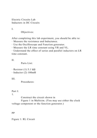
  • 1. Electric Circuits Lab Inductors in DC Circuits I. Objectives: After completing this lab experiment, you should be able to: · Measure the resistance and Inductance. · Use the Oscilloscope and Function generator. · Measure the LR time constant using VR and VL. · Understand the effect of series and parallel inductors on LR time constant. II. Parts List: · Resistor (1) 5.1 kΩ · Inductor (2) 100mH III. Procedures: Part I: 1. Construct the circuit shown in Figure 1 in Multisim. (You may use either the clock voltage component or the function generator.) PP Figure 1: RL Circuit
  • 2. 2. Connect Channel A of the oscilloscope across the resistor and Channel B across the inductor. 3. Set the voltage source to 5VPP; 300 Hz, Square wave, 50% duty cycle 4. You should be able to see the waveform as shown below. (Use Volts/Div and Time/DIV settings to adjust the signal) Figure 2. Voltage across the inductor and resistor 5. Calculate the time constant of an LR circuit. Record the result in Table 1 below under the calculated value. Calculated value Measured value using VL Measured value using VR 19.6 us 20.319 us 20.398 us Table 1: Calculated and measured time constant values 6. Turn on the cursors on the oscilloscope 7. Measuring the time constant with VL: (shown in Figure 3)
  • 3. i. Set Channel A to “0” to turn off Channel A signal. ii. Measure the peak value of the voltage across the resistor, by placing one of the cursors at the peak point _____5.002 V____. iii. Calculate the 37% of the above value ___1.85V______. iv. Place the second cursor at the voltage calculated above in step (iii). v. Observe the change in time (T2-T1) value on the scope, which is the value of one time constant. vi. Record the T2-T1 value in Table 1 above under measured value using VL. Figure 3: Measuring RL time constant using VL example (L = 150 mH) Note: your scope screen will be different 8. Set Channel B to “0” to turn it off. 9. Set Channel A to “AC” 10. Adjust the Trigger settings, if needed, and you should be
  • 4. able to see the waveform as shown below. (Use Volts/Div and Time/DIV knobs to adjust the signal) Figure 4: Voltage across the resistor 11. Measuring the time constant: (shown in Figure 5) i. Measure the peak value of the signal, by placing one of the cursors (T1) at the peak point and the other cursor (T2) at the negative peak. Calculate the total peak-to-peak voltage (T1-T2) _4.998V________. ii. Calculate the 63% of the above value __3.15V_______. iii. Place the second cursor (T2) at the negative peak value plus the step (ii) value above . iv. Place T1 at the negative peak just before the signal begins to rise. vii. Observe the dT (T2-T1) value on the scope, which is one time constant. viii.
  • 5. Record the result in Table 1 above under measured value using VR. Figure 5: Measuring RL time constant using VR example (L = 150 mH) Note: your scope screen will be different Part II: 12. Place two inductors in series as shown below. Figure 6: Series Inductors 13. Calculate the total inductance value and record the results in Table 2 (Calculated) below. 14. Measure the total inductance value. (If you have the proper measuring device to do so). Use the following procedure to measure the inductance in Multisim if you do not have the proper measuring device. i. Connect the Impedance Meter (Simulate >>Instruments>>LabView Instruments>>Impedance Meter) as shown in
  • 6. Figure 7. ii. Measure the inductive reactance, XL, as shown in Figure 7 . iii. Calculate the inductance using the equation. and record the value in Table 2 (Measured). Calculated Value Measured Value Inductance 200 199.99 Table 2: Series Inductors Figure 7. Impedance Meter in Multisim Example 15. Build the circuit in Figure 8. Figure 8: RL circuit with series Inductors 16. Calculate the new LR time constant. Record the result in
  • 7. Table 3 below. 17. Connect Channel A of the oscilloscope across the resistor. 18. Adjust the Trigger, if needed, and you should be able to see the waveform as shown below. (Use Volts/Div and Time/DIV knobs to adjust the signal) Figure 9: Voltage across the resistor 19. Use the cursors on the oscilloscope to measure the time constant (refer to step 11). Record the result in Table 3 below under measured value. Calculated value Measured value using VR 40 us 41.276 us Table 3: Calculated and measured time constant values Part III: 20. Place two inductors in parallel as shown below. ( Note: The 0.001 Ω resistor is ONLY required for simulation in Multisim. Without the resistor, the mathematical model will not converge.)
  • 8. Figure 10: Parallel Inductors 21. Calculate the total inductance value and record the results in Table 4 (Calculated). Calculated value Measured value Inductance 50 50 Table 4: Parallel Inductors 22. Measure the total parallel inductance value. (If you have the proper device to do so). Use the following procedure to measure the inductance in Multisim if you do not have the proper measuring device. i. Connect the Impedance Meter (Simulate >>Instruments>>LabView Instruments>>Impedance Meter). ii. Measure the inductive reactance, XL 18.8496 . iii. Calculate the inductance using the equation and record the value in
  • 9. Table 4 (Measured). 23. Build the following circuit. ( Note: The 0.001 Ω resistor is ONLY required for simulation in Multisim. Without the resistor, the mathematical model will not converge.) Figure 11: RL circuit with parallel Inductors 24. Calculate the new LR time constant. Record the result in Table 5 below. 25. Connect Channel A of the oscilloscope across the resistor. 26. You should be able to see the waveform as shown below. (Use Volts/Div and Time/DIV knobs to adjust the signal) Figure 12: Voltage across the resistor 27. Use the cursors on the oscilloscope to measure the time constant (refer to step 11). Record the result in Table 5 below under measured value. Calculated value Measured value using VR
  • 10. 8.3 11.183 Table 5: Calculated and measured time constant values 1 image4.png image5.png image6.png image7.png image8.png image9.png image10.png image11.png image12.emf Week2 Circuit 1.ms14 image13.emf Week2 Circuit 2.ms14 image14.emf Week2 Circuit 3.ms14 image15.png image16.png image17.png image18.png image19.png image20.png image21.png image1.png image2.png
  • 11. image3.png ELECTRIC CIRCUITS I METRIC PREFIX TABLE Metric Prefix Symbol Multiplier (Traditional Notation) Expo- nential Description Yotta Y 1,000,000,000,000,000,000,000,000 1024 Septillion Zetta Z 1,000,000,000,000,000,000,000 1021 Sextillion Exa E 1,000,000,000,000,000,000 1018 Quintillion Peta P 1,000,000,000,000,000 1015 Quadrillion Tera T 1,000,000,000,000
  • 14. zepto z 1/1,000,000,000,000,000,000,000 10-21 Sextillionth yocto y 1/1,000,000,000,000,000,000,000,000 10-24 Septillionth 4-BAND RESISTOR COLOR CODE TABLE BAND COLOR DIGIT Band 1: 1st Digit Band 2: 2nd Digit Band 3: Multiplier (# of zeros following 2nd digit) Black 0
  • 16. COLOR DIGIT Band 1: 1st Digit Band 2: 2nd Digit Band 3: 3rd Digit Band 4: Multiplier (# of zeros following 3rd digit) Black 0 Brown 1 Red 2 Orange 3 Yellow 4 Green 5 Blue 6 Violet
  • 17. 7 Gray 8 White 9 Gold 0.1 SILVER 0.01 Band 5: Tolerance Gold ± 5% SILVER ± 10% EET Formulas & Tables Sheet Page 1 of 21 UNIT 1: FUNDAMENTAL CIRCUITS CHARGE Where: Q = Charge in Coulombs (C) Note: 1 C = Total charge possessed by 6.25x10¹⁸ electrons VOLTAGE
  • 18. Where: V = Voltage in Volts (V) W = Energy in Joules (J) Q = Charge in Coulombs (C) CURRENT Where: I = Current in Amperes (A) Q = Charge in Coulombs (C) t = Time in seconds (s) OHM’S LAW Where: I = Current in Amperes (A) V = Voltage in Volts (V) R = Resistance in Ohms (Ω) RESISTIVITY Where: ρ = Resistivity in Circular Mil – Ohm per Foot (CM-Ω/ft) A = Cross-sectional area in Circular Mils (CM) R = Resistance in Ohms (Ω) ɭ = Length in Feet (ft) Note: CM: Area of a wire with a 0.001 inch (1 mil) diameter
  • 19. CONDUCTANCE Where: G = Conductance in Siemens (S) R = Resistance in Ohms (Ω) CROSS-SECTIONAL AREA Where: A = Cross-sectional area in Circular Mils (CM) d = Diameter in thousandths of an inch (mils) ENERGY Where: W = Energy in Joules (J). Symbol is an italic W. P = Power in Watts (W). Unit is not an italic W. t = Time in seconds (s) Note:
  • 20. 1 W = Amount of power when 1 J of energy is used in 1 s POWER Where: P = Power in Watts (W) V = Voltage in Volts (V) I = Current in Amperes (A) Note: Ptrue = P in a resistor is also called true power OUTPUT POWER Where: POUT = Output power in Watts (W) PIN = Input power in Watts (W) PLOSS = Power loss in Watts (W) POWER SUPPLY EFFICIENCY Where: POUT = Output power in Watts (W) PIN = Input power in Watts (W) Efficiency = Unitless value Note: Efficiency expressed as a percentage:
  • 21. UNIT 2: SERIES CIRCUITS (R1, R2, , Rn) TOTAL RESISTANCE Where: RT = Total series resistance in Ohms (Ω) Rn = Circuit’s last resistor in Ohms (Ω) KIRCHHOFF’S VOLTAGE LAW Where: VS = Voltage source in Volts (V) Vn = Circuit’s last voltage drop in Volts (V) VOLTAGE – DIVIDER Where: Vx = Voltage drop in Ohms (Ω) Rx = Resistance where Vx occurs in Ohms (Ω) RT = Total series resistance in Ohms (Ω)
  • 22. VS = Voltage source in Volts (V) TOTAL POWER Where: PT = Total power in Watts (W) Pn = Circuit’s last resistor’s power in Watts (W) UNIT 3: PARALLEL CIRCUITS (R1||R2||||Rn) TOTAL RESISTANCE Where: RT = Total parallel resistance in Ohms (Ω) Rn = Circuit’s last resistor in Ohms (Ω) TOTAL RESISTANCE - TWO RESISTORS IN PARALLEL Where: RT = Total parallel resistance in Ohms (Ω)
  • 23. TOTAL RESISTANCE - EQUAL-VALUE RESISTORS Where: RT = Total parallel resistance in Ohms (Ω) R = Resistor Value in Ohms (Ω) n = Number of equal value resistors (Unitless) UNKNOWN RESISTOR Where: Rx = Unknown resistance in Ohms (Ω) RA = Known parallel resistance in Ohms (Ω) RT = Total parallel resistance in Ohms (Ω) KIRCHHOFF’S CURRENT LAW Where: n = Number of currents into node (Unitless) m = Number of currents going out of node (Unitless) CURRENT – DIVIDER
  • 24. Where: Ix = Branch “x” current in Amperes (A) RT = Total parallel resistance in Ohms (Ω) Rx = Branch “x” resistance in Ohms (Ω) IT = Total current in Amperes (A) TWO-BRANCH CURRENT – DIVIDER Where: I1 = Branch “1” current in Amperes (A) R2 = Branch “2” resistance in Ohms (Ω) R1 = Branch “1” resistance in Ohms (Ω) IT = Total current in Amperes (A) TOTAL POWER Where: PT = Total power in Watts (W) Pn = Circuit’s last resistor’s power in Watts (W) OPEN BRANCH RESISTANCE Where: ROpen = Resistance of open branch in Ohms (Ω) RT(Meas) = Measured resistance in Ohms (Ω) GT(Calc) = Calculated total conductance in Siemens (S) GT(Meas) = Measured total conductance in Siemens (S) Note: GT(Meas) obtained by measuring total resistance, RT(Meas)
  • 25. UNIT 4: SERIES - PARALLEL CIRCUITS BLEEDER CURRENT Where: IBLEEDER = Bleeder current in Amperes (A) IT = Total current in Amperes (A) IRL1 = Load resistor 1 current in Amperes (A) IRL2 = Load resistor 2 current in Amperes (A) THERMISTOR BRIDGE OUTPUT Where: = Change in output voltage in Volts (V) = Change in thermal resistance in Ohms (Ω) VS = Voltage source in Volts (V) R = Resistance value in Ohms (Ω) UNKNOWN RESISTANCE IN A WHEATSTONE BRIDGE Where: RX = Unknown resistance in Ohms (Ω) RV = Variable resistance in Ohms (Ω) R2 = Resistance 2 in Ohms (Ω) R4 = Resistance 4 in Ohms (Ω)
  • 26. UNIT 5: MAGNETISM AND ELECTROMAGNETISM MAGNETIC FLUX DENSITY Where: B = Magnetic flux density in Tesla (T) = Flux in Weber (Wb) (Greek letter Phi) A = Cross-sectional area in square meters (m2) Note: Tesla (T) equals a Weber per square meter (Wb/m2) RELATIVE PERMEABILITY Where: = Relative permeability (Unitless) (Greek letter Mu)
  • 27. = Permeability in Webers per Ampere-turn · meter (Wb/At·m) = Vacuum permeability in Webers per Ampere- turn · meter (Wb/At·m) Note: = Wb/ At·m RELUCTANCE Where: R = Reluctance in Ampere-turn per Weber (At/Wb) ɭ = Length of magnetic path in meters (m) µ = Permeability in Weber per Ampere-turn · meter (Wb/At · m) A = Cross-sectional area in meters squares (m2) MAGNETOMOTIVE FORCE Where: Fm = Magnetomotive force (mmf) in Ampere-turn (At) N = Number of Turns of wire (t) I = Current in Amperes (A) MAGNETIC FLUX
  • 28. Where: = Flux in Weber (Wb) Fm = Magnetomotive force in Ampere-turn (At) R = Reluctance in Ampere-turn per Weber (At/Wb) MAGNETIC FIELD INTENSITY Where: H = Magnetic field intensity in Amperes-turn per meter (At/m) Fm = Magnetomotive force in Ampere-turn (At) ɭ = Length of material in meters (m) INDUCED VOLTAGE Where: vind = Induced voltage in Volts (V) B = Magnetic flux density in Tesla (T) ɭ = Length of the conductor exposed to the magnetic field in meters (m) v = Relative velocity in meters per second (m/s) Note: Tesla (T) equals a Weber per square meter (Wb/m2) FARADAY’S LAW
  • 29. Where: vind = Induced voltage in Volts (V) N = Number of turns of wire in the coil (Unitless) = Rate of change of magnetic field with respect to the coil in Webers per second (Wb/s) ELECTRIC CIRCUITS II UNIT 1: ALTERNATE CURRENT & INDUCTORS ALTERNATE CURRENT FREQUENCY & PERIOD Where: f = Frequency in Hertz (Hz) T = Period in Seconds (s) Note: 1 Hertz = 1 cycle per 1 second PEAK TO PEAK VOLTAGE Where: Vpp = Peak to peak voltage in Volts (V) Vp = Peak voltage in Volts (V) ROOT MEAN SQUARE (RMS) VOLTAGE
  • 30. Where: Vrms = Root mean square voltage in Volts (V) Vp = Peak voltage in Volts (V) HALF-CYCLE AVERAGE VOLTAGE Where: Vavg = Half-cycle average voltage in Volts (V) Vp = Peak voltage in Volts (V) RADIAN & DEGREE CONVERSION Where: Rad = Number of radians in Rad (rad) Degrees = Number of degrees in Degrees (0) Note: = 3.1416 (Greek letter Pi) GENERATOR OUTPUT FREQUENCY Where: f = Frequency in Hertz (Hz)
  • 31. Number of pole pairs = Number of pole pairs (Unitless) rps = Revolutions per second in Revolutions per Second (rps) PEAK TO PEAK CURRENT Where: Ipp = Peak to peak current in Amperes (A) Ip = Peak current in Amperes (A) ROOT MEAN SQUARE (RMS) CURRENT Where: Irms = Root mean square current in Amperes (A) Ip = Peak current in Amperes (A) HALF-CYCLE AVERAGE CURRENT Where: Iavg = Half-cycle average current in Amperes (A) Ip = Peak current in Amperes (A) SINE WAVE GENERAL FORMULA Where:
  • 32. y = Instantaneous voltage or current value at angle in Volts or Amperes (V or A) (Greek letter Theta) A = Maximum voltage or current value in Volts or Amperes (V or A) = Angle where given instantaneous voltage or current value exists SINE WAVE LAGGING THE REFERENCE Where: y = Instantaneous voltage or current value at angle in Volts or Amperes (V or A) A = Maximum voltage or current value in Volts or Amperes (V or A) = Angle where given instantaneous voltage or current value exists = Angle sine wave is shifted right (lagging) of reference (Greek letter Phi) ANGULAR VELOCITY Where: = Angular velocity in Radians per second (rad/s) (Small Greek letter omega) f = Frequency in Hertz (Hz) Note: = 3.1416 SINE WAVE VOLTAGE
  • 33. Where: v = Sinusoidal voltage in Volts (V) Vp = Peak voltage in Volts (V) f = Frequency in Hertz (Hz) t = Time in Seconds (s) Note: = 3.1416 PULSE WAVEFORM AVERAGE VALUE Where: vavg = Pulse waveform average value in Volts (V) baseline = Baseline in Volts (V) duty cycle = Percent duty cycle in Percent/100% (Unitless) Amplitude = Amplitude in Volts (V) SINE WAVE LEADING THE REFERENCE Where: y = Instantaneous voltage or current value at angle in Volts or Amperes (V or A) A = Maximum voltage or current value in Volts or Amperes (V or A) = Angle where given instantaneous voltage or current value exists = Angle sine wave is shifted left (leading) of
  • 34. reference PHASE ANGLE Where: = Angle sine wave is shifted in Radians (rad) = Angular velocity in Radians per second (rad/s) t = Time in Seconds (s) DUTY CYCLE Where: Percent duty cycle = Percent duty cycle in Percentage (%) tw = Pulse width in Seconds (s) T = Period in Seconds (s) F = Frequency in Hertz (Hz)
  • 35. INDUCTORS INDUCED VOLTAGE Where: vind = Induced voltage in Volts (V) L = Inductance in Henries (H) = Time rate of change of the current in Amperes per second (A/s) INDUCTANCE OF A COIL Where: L = Inductance of a coil in Henries (H) N = Number of turns of wire (Unitless) = Permeability in Henries per meter (H/m) A = Cross-sectional area in Meters squared (m2) = Core length in Meters (m) Notes: Permeability in H/m is equal to Wb/At·m Non-magnetic core = Permeability of a vacuum, µ0 µ0 = 4 x 10⁻⁷ H/m
  • 36. RL TIME CONSTANT Where: = RL time constant in Seconds (s) (Greek letter Tau) L = Inductance in Henries (H) R = Resistance in Ohms (Ω) GENERAL EXPONENTIAL VOLTAGE FORMULA Where: v = Instantaneous voltage at time, t, in Volts (V) VF = Voltage final value in Volts (V) Vi = Voltage initial value in Volts (V) R = Resistance in Ohms (Ω) t = Time in Seconds (s) L = Inductance in Henries (H) INDUCTOR ENERGY STORAGE Where: W = Energy in Joules (J) L = Inductance in Henries (H) I = Current in Amperes (A) TOTAL INDUCTANCE - SERIES
  • 37. Where: LT = Total series inductance in Henries (H) Ln = Circuit’s last inductor in Henries (H) TOTAL INDUCTANCE – PARALLEL Where: LT = Total parallel inductance in Henries (H) Ln = Circuit’s last inductor in Henries (H) RL CIRCUIT CURRENT INCREASE AND DECREASE FOR GIVEN NUMBER OF TIME CONSTANTS # of Time Constants Approx % of Final Current Approx % of Initial Charge 1 63 37 2 86 14 3 95 5 4 98 2 5 99 Considered 100% 1
  • 38. Considered 0% GENERAL EXPONENTIAL CURRENT FORMULA Where: i = Instantaneous current at time, t, in Amperes (A) IF = Current final value in Amperes (A) Ii = Current initial value in Amperes (A) R = Resistance in Ohms (Ω) t = Time in Seconds (s) L = Inductance in Henries (H) INDUCTIVE REACTANCE Where: XL = Inductive reactance in Ohms (Ω) f = Frequency in Hertz (Hz) L = Inductance in Henries (H) Note: = 3.1416 (Greek letter “Pi”) INDUCTOR REACTIVE POWER Where: Pr = Reactive Power in Watts (W) Vrms = Voltage rms in Volts (V) Irms = Current rms in Amperes (A) XL = Inductive reactance in Ohms (Ω)
  • 39. UNIT 2: RL CIRCUITS SERIES RL CIRCUIT IMPEDANCE IN RECTANGULAR FORM Where: Z = Impedance in Ohms (Ω) R = Resistance in Ohms (Ω) XL = Inductive reactance in Ohms (Ω) Note: Bold letters represent complete phasor quantities. For example, “ Z” in the formula above VOLTAGE IN RECTANGULAR FORM Where: Vs = Voltage in Volts (V) VR = Resistor voltage in Volts (V) VL = Inductor voltage in Volts (V) INDUCTOR TRUE POWER Where: Ptrue = True Power in Watts (W) Irms = Current rms in Amperes (A) RW = Winding resistance in Ohms (Ω)
  • 40. COIL QUALITY FACTOR Where: Q = Coil quality factor (Unitless) XL = Inductive reactance in Ohms (Ω) RW = Winding resistance of the coil or the resistance in series with the coil in Ohms (Ω) Note: Circuit Q and the coil Q are the same when the resistance is only the coil winding resistance IMPEDANCE IN POLAR FORM Where: Z = Impedance in Ohms (Ω) R = Resistance in Ohms (Ω) XL = Inductive reactance in Ohms (Ω) Note: = Magnitude = Phase Angle VOLTAGE IN POLAR FORM Where: Vs = Voltage in Volts (V) VR = Resistor voltage in Volts (V)
  • 41. VL = Inductor voltage in Volts (V) LEAD CIRCUIT ANGLE BETWEEN VOLTAGE IN & OUT Where: = Angle between voltage in and out in Degrees (0) R = Resistance in Ohms (Ω) XL = Inductive reactance in Ohms (Ω) OUTPUT VOLTAGE MAGNITUDE Where: Vout = Voltage output in Volts (V) XL = Inductive reactance in Ohms (Ω) R = Resistance in Ohms (Ω) LAG CIRCUIT ANGLE BETWEEN VOLTAGE IN & OUT Where: = Angle between voltage in and out in Degrees (0) XL = Inductive reactance in Ohms (Ω) R = Resistance in Ohms (Ω) OUTPUT VOLTAGE MAGNITUDE
  • 42. Where: Vout = Output voltage in Volts (V) R = Resistance in Ohms (Ω) XL = Inductive reactance in Ohms (Ω) Vin = Input voltage in Volts (V) PARALLEL RL CIRCUIT TOTAL 2-COMPONENT IMPEDANCE Where: Z = Total 2-component impedance in Ohms (Ω) R = Resistance in Ohms (Ω) XL = Inductive reactance in Ohms (Ω) CURRENT IN POLAR FORM Where: Itot = Total current in Amperes (A) IR = Resistor current in Amperes (A) IL = Inductor current in Amperes (A) TOTAL ADMITTANCE Where:
  • 43. Y = Total admittance in Siemens (S) G = Conductance in Siemens (S) BL = Inductive Susceptance in Siemens (S) Note: CURRENT IN RECTANGULAR FORM Where: Itot = Total current in Amperes (A) IR = Resistor current in Amperes (A) IL = Inductor current in Amperes (A) PARALLEL TO SERIES FORM CONVERSION Where: Req = Resistance in Ohms (Ω) Z = Impedance in Ohms (Ω) XL = Inductive reactance in Ohms (Ω) = Angle where given instantaneous voltage or current value exists POWER RL CIRCUIT REACTIVE POWER Where: Pr = Reactive power in Volt-Ampere Reactive (VAR) Itot = Total current in Amperes (A) XL = Inductive reactance in Ohms (Ω)
  • 44. UNIT 3: CAPACITORS CAPACITANCE Where: C = Capacitance in Farads (F) Q = Charge in Coulombs (C) V = Voltage in Volts (V) ENERGY STORED IN A CAPACITOR Where: W = Energy in Joules (J) C = Capacitance in Farads (F) V = Voltage in Volts (V) DIELECTRIC CONSTANT (RELATIVE PERMITTIVITY) Where: = Dielectric constant (Unitless) (Greek letter Epsilon) = Absolute permittivity of a material in Farads per meter (F/m) = Absolute permittivity of a vacuum in Farads per meter (F/m) Note: = 8.85 x 10⁻¹² F/m
  • 45. CAPACITANCE Where: C = Capacitance in Farads (F) A = Plate area in Meters squared (m2) = Dielectric constant (Unitless) d = Plate separation in Meters (m) Note: If d is in mils, 1 mil = 2.54 x 10⁻⁵ meters SERIES CAPACITORS TOTAL CHARGE Where: QT = Total charge in Coulombs (C) Qn = Circuit’s last capacitor charge in Coulombs (C) TOTAL CAPACITANCE Where: CT = Total series capacitance in Farads (F) Cn = Circuit’s last capacitor’s capacitance in Farads (F) TOTAL CAPACITANCE - TWO CAPACITORS
  • 46. Where: CT = Total series capacitance in Farads (F) VOLTAGE ACROSS A CAPACITOR Where: Vx = Voltage drop in Volts (V) CT = Total series capacitance in Farads (F) Cx = Capacitor x’s capacitance in Farads (F) VT = Total voltage in Volts (V) TOTAL CAPACITANCE - EQUAL-VALUE CAPACITORS Where: CT = Total series capacitance in Farads (F) n = Number of equal value capacitors (Unitless) PARALLEL CAPACITORS
  • 47. TOTAL CHARGE Where: QT = Total charge in Coulombs (C) Qn = Circuit’s last capacitor charge in Coulombs (C) TOTAL CAPACITANCE - EQUAL-VALUE CAPACITORS Where: CT = Total series capacitance in Farads (F) n = Number of equal value capacitors (Unitless) CAPACITORS IN DC CIRCUITS RC TIME CONSTANT Where: = Time constant in Seconds (s) R = Resistance in Ohms (Ω) C = Capacitance in Farads (F) TOTAL CAPACITANCE
  • 48. Where: CT = Total series capacitance in Farads (F) Cn = Circuit’s last capacitor’s capacitance in Farads (F) RC CIRCUIT CURRENT INCREASE AND DECREASE FOR GIVEN NUMBER OF TIME CONSTANTS # of Time Constants Approx % of Final Current Approx % of Initial Charge 1 63 37 2 86 14 3 95 5 4 98 2 5
  • 49. 99 Considered 100% 1 Considered 0% GENERAL EXPONENTIAL VOLTAGE FORMULA Where: v = Instantaneous voltage at time, t, in Volts (V) VF = Voltage final value in Volts (V) Vi = Voltage initial value in Volts (V) t = Time in Seconds (s) = Time constant in Seconds (s) CHARGING TIME TO A SPECIFIED VOLTAGE Where: t = Time in Seconds (s) R = Resistance in Ohms (Ω) C = Capacitance in Farads (F) v = Specified voltage level in Volts (V) VF = Final voltage level in Volts (V) Note: Assumes Vi = 0 Volts GENERAL EXPONENTIAL CURRENT FORMULA Where: i = Instantaneous current at time, t, in Amperes (A) IF = Current final value in Amperes (A)
  • 50. Ii = Current initial value in Amperes (A) t = Time in Seconds (s) = Time constant in Seconds (s) DISCHARGING TIME TO A SPECIFIED VOLTAGE Where: t = Time in Seconds (s) R = Resistance in Ohms (Ω) C = Capacitance in Farads (F) v = Specified voltage level in Volts (V) Vi = Initial voltage level in Volts (V) Note: Assumes VF = 0 Volts CAPACITORS IN AC CIRCUITS INSTANTANEOUS CAPACITOR CURRENT Where: i = Instantaneous current in Amperes (A) C = Capacitance in Farads (F) = Instantaneous rate of change of the voltage across the capacitor in Volts per second (V/s) CAPACITOR REACTIVE POWER
  • 51. Where: Pr = Reactive Power in Volt-Ampere Reactive (VAR) Vrms = Voltage rms in Volts (V) Irms = Current rms in Amperes (A) XC = Capacitive reactance in Ohms (Ω) CAPACITIVE REACTANCE Where: XC = Capacitive reactance in Ohms (Ω) f = Frequency in Hertz (Hz) C = Capacitance in Farads (F) Note: = 3.1416 (Greek letter “Pi”) SWITCHED-CAPACITORS CIRCUITS AVERAGE CURRENT
  • 52. Where: I1(avg) = Instantaneous current in Amperes (A) C = Capacitance in Farads (F) V1 = Voltage 1 in Volts (V) V2 = Voltage 2 in Volts (V) T = Period of time in Seconds (s) UNIT 4: RC CIRCUITS RC SERIES CIRCUITS IMPEDANCE IN RECTANGULAR FORM Where: Z = Impedance in Ohms (Ω) R = Resistance in Ohms (Ω) XC = Capacitive reactance in Ohms (Ω) OHM’S LAW Where: I = Current in Amperes (A) Z = Impedance in Ohms (Ω) V = Voltage in Volts (V) VOLTAGE IN RECTANGULAR FORM Where: Vs = Voltage in Volts (V)
  • 53. VR = Resistor voltage in Volts (V) VC = Capacitor voltage in Volts (V) LEAD CIRCUIT ANGLE BETWEEN VOLTAGE IN & OUT Where: = Angle between voltage in and out in Degrees (0) XC = Capacitive reactance in Ohms (Ω) R = Resistance in Ohms (Ω) EQUIVALENT RESISTANCE Where: R = Equivalent resistance in Ohms (Ω) T = Period of time in Seconds (s) C = Capacitance in Farads (F) f = Frequency in Hertz (Hz) IMPEDANCE IN POLAR FORM Where: Z = Impedance in Ohms (Ω) R = Resistance in Ohms (Ω) XC = Capacitive reactance in Ohms (Ω)
  • 54. VOLTAGE IN POLAR FORM Where: Vs = Voltage in Volts (V) VR = Resistor voltage in Volts (V) VC = Capacitor voltage in Volts (V) OUTPUT VOLTAGE MAGNITUDE Where: Vout = Voltage output in Volts (V) R = Resistance in Ohms (Ω) XC = Capacitive reactance in Ohms (Ω) LAG CIRCUIT ANGLE BETWEEN VOLTAGE IN & OUT Where: = Angle between voltage in and out in Degrees (0) R = Resistance in Ohms (Ω) XC = Capacitive reactance in Ohms (Ω)
  • 55. RC PARALLEL CIRCUITS TOTAL 2-COMPONENT IMPEDANCE Where: Z = Total 2-component impedance in Ohms (Ω) R = Resistance in Ohms (Ω) XC = Capacitive reactance in Ohms (Ω) OHM’S LAW Where: I = Current in Amperes (A) V = Voltage in Volts (V) Y = Admittance in Siemens (S) CURRENT IN RECTANGULAR FORM Where: Itot = Total current in Amperes (A) IR = Resistor current in Amperes (A) IC = Capacitor current in Amperes (A) PARALLEL TO SERIES FORM CONVERSION Where: Req = Resistance in Ohms (Ω) Z = Impedance in Ohms (Ω)
  • 56. XC = Capacitive reactance in Ohms (Ω) = Angle where given instantaneous voltage or current value exists OUTPUT VOLTAGE MAGNITUDE Where: Vout = Voltage output in Volts (V) XC = Capacitive reactance in Ohms (Ω) R = Resistance in Ohms (Ω) TOTAL ADMITTANCE Where: Y = Total admittance in Siemens (S) G = Conductance in Siemens (S) BC = Capacitive susceptance in Siemens (S) Note: CURRENT IN POLAR FORM Where: Itot = Total current in Amperes (A) IR = Resistor current in Amperes (A) IC = Capacitor current in Amperes (A) RC SERIES –PARALLEL CIRCUITS
  • 57. PHASE ANGLE Where: Req = Resistance in Ohms (Ω) Z = Impedance in Ohms (Ω) XC = Capacitive reactance in Ohms (Ω) = Angle where given instantaneous voltage or current value exists POWER APPARENT POWER Where: Pa = Apparent power in Volt-ampere (VA) I = Current in Amperes (A) Z = Impedance in Ohms (Ω) POWER FACTOR Where: PF = Power Factor (Unitless) = Phase angle in Degrees (0) OSCILLATOR AND FILTER OSCILLATOR OUTPUT FREQUENCY Where: fr = Output frequency in Hertz (Hz) R = Resistance in Ohms (Ω) C = Capacitance in Farads (F) Note: = 3.1416 UNIT 5: RLC CIRCUITS AND PASSIVE FILTERS
  • 58. RLC SERIES CIRCUITS TOTAL REACTANCE Where: Xtot = Total reactance in Ohms (Ω) XL = Inductive reactance in Ohms (Ω) XC = Capacitive reactance in Ohms (Ω) TOTAL IMPEDANCE IN POLAR FORM Where: Z = Total impedance in Ohms (Ω) R = Resistance in Ohms (Ω) XL = Inductive reactance in Ohms (Ω) XC = Capacitive reactance in Ohms (Ω) Xtot = Total reactance in Ohms (Ω) Note: When XL > XC, the angle is positive When XC > XL, the angle is negative TRUE POWER Where: Ptrue = True power in Watts (W) V = Voltage in Volts (V) I = Current in Amperes (A) = Phase angle in Degrees (0)
  • 59. FILTER CUTOFF FREQUENCY Where: fc = Cutoff frequency in Hertz (Hz) R = Resistance in Ohms (Ω) C = Capacitance in Farads (F) Note: = 3.1416 TOTAL IMPEDANCE IN RECTANGULAR FORM Where: Z = Total impedance in Ohms (Ω) R = Resistance in Ohms (Ω) XL = Inductive reactance in Ohms (Ω) XC = Capacitive reactance in Ohms (Ω) RESONANT FREQUENCY Where: fr = Resonant frequency in Hertz (Hz) L = Inductance in Henries (H) C = Capacitance in Farads (F) Note: At resonance, XL = XC and the j terms cancel = 3.1416 RLC PARALLEL CIRCUITS TOTAL CURRENT Where: Itot = Total current in Amperes (A)
  • 60. IR = Resistor current in Amperes (A) IC = Capacitor current in Amperes (A) IL = Inductor current in Amperes (A) ICL = Total current into the L and C branches in Amperes (A) RLC PARALLEL RESONANCE RESONANT FREQUENCY - IDEAL Where: fr = Resonant frequency in Hertz (Hz) L = Inductance in Henries (H) C = Capacitance in Farads (F) Note: At resonance, XL = XC and Zr = = 3.1416 CURRENT AND PHASE ANGLE
  • 61. Where: Itot = Total current in Amperes (A) VS = Voltage source in Volts (V) Zr = Impedance at resonance in Ohms (Ω) RESONANT FREQUENCY - PRECISE Where: fr = Resonant frequency in Hertz (Hz) RW = Winding resistance in Ohms (Ω) C = Capacitance in Farads (F) L = Inductance in Henries (H) Note: = 3.1416 RLC SERIES – PARALLEL CIRCUITS SERIES-PARALLEL TO PARALLEL CONVERSION EQUIVALENT INDUCTANCE Where: Leq = Equivalent inductance in Henries (H) L = Inductance in Henries (H) Q = Coil quality factor (Unitless)
  • 62. EQUIVALENT PARALLEL RESISTANCE Where: Rp(eq) = Equivalent parallel resistance in Ohms (Ω) RW = Winding resistance in Ohms (Ω) Q = Coil quality factor (Unitless) NON-IDEAL TANK CIRCUIT TOTAL IMPEDANCE AT RESONANCE Where: ZR = Total impedance in Ohms (Ω) RW = Resistance in Ohms (Ω) Q = Coil quality factor (Unitless) SPECIAL TOPICS RESONANT CIRCUIT BANDWIDTH BANDWIDTH Where: BW = Bandwidth in Hertz (Hz) f2 = Upper critical frequency at Z=0.707·Zmax in Hertz (Hz) f1 = Lower critical frequency at Z=0.707·Zmax in Hertz (Hz)
  • 63. BANDWIDTH AND QUALTIY FACTOR Where: BW = Bandwidth in Hertz (Hz) fr = Center (resonant) frequency in Hertz (Hz) Q = Coil quality factor (Unitless) PASSIVE FILTERS POWER RATIO IN DECIBELS Where: dB = Power ratio in decibels (dB) Pout = Output power in Watts (W) Pin = Input power in Watts (W) OVERALL QUALITY FACTOR WITH AN EXTERNAL LOAD Where: QO = Overall quality factor (Unitless) Rp(tot)= Total parallel equivalent resistance in Ohms (Ω) XL = Inductive reactance in Ohms (Ω) CENTER (RESONANT) FREQUENCY Where: fr = Center (resonant) frequency in Hertz (Hz) f1 = Lower critical frequency at Z=0.707·Zmax in Hertz (Hz)
  • 64. f2 = Upper critical frequency at Z=0.707·Zmax in Hertz (Hz) VOLTAGE RATIO IN DECIBELS Where: dB = Power ratio in decibels (dB) Vout = Output voltage in Volts (V) Vin = Input voltage in Volts (V) LOW-PASS & HIGH-PASS FILTERS RC FILTERS Where: fC = Filter critical frequency in Hertz (Hz) R = Resistance in Ohms (Ω) C = Capacitance in Farads (F) Note:
  • 65. = 3.1416 At fC, Vout = (0.707)·Vin SERIES RESONANT BAND-PASS FILTER Where: BW = Bandwidth in Hertz (Hz) f0 = Center frequency in Hertz (Hz) Q = Coil quality factor (Unitless) RL FILTERS Where: fc = Filter critical frequency in Hertz (Hz) L = Inductance in Henries (H) R = Resistance in Ohms (Ω) Note: = 3.1416 At fC, Vout = (0.707)·Vin GENERAL INFORMATION AREA AND VOLUMES AREAS
  • 66. CIRCLE AREA Where: A = Circle area in meters squared (m2) r = Radius in meters (m) Note: = 3.1416 RECTANGULAR AND POLAR FORMS RECTANGULAR FORM Where: A = Coordinate value on real axis (Horizontal Plane)
  • 67. j = j operator B = Coordinate value on imaginary axis (Vertical Plan) Note: “j operator” prefix indicates designated coordinate value is on imaginary axis. COMPLEX PLANE AND RECTANGULAR FORM PHASOR +A Quadrant 1 Quadrant 3 Quadrant 4 -A +jB -jB (A + jB) (A - jB) (-A + jB) (-A - jB) Quadrant 2 00/3600 1800 900 2700 POLAR FORM Where: C = Phasor magnitude = Phasor angle relative to the positive real axis
  • 68. COMPLEX PLANE AND POLAR FORM PHASOR Real Axis Quadrant 1 Quadrant 3 Quadrant 4 +j -j Length = Magnitude - Quadrant 2 + RECTANGULAR TO POLAR CONVERSION Where: A = Coordinate value on real axis (Horizontal Plane) j = j operator B = Coordinate value on imaginary axis (Vertical Plan) C = Phasor magnitude = Phasor angle relative to the positive real axis Note: To calculate C: To calculate in Quadrants 1 and 4 (A is positive): Use +B for +B values, -B for –B values To calculate in Quadrants 2 and 3 (A is negative): Use for +B values
  • 69. Use for –B values POLAR TO RECTANGULAR CONVERSION Where: C = Phasor magnitude = Phasor angle relative to the positive real axis A = Coordinate value on real axis (Horizontal Plane) j = j operator B = Coordinate value on imaginary axis (Vertical Plan) Note: To calculate A: To calculate B: Electric Circuits Lab Instructor: ----------- Lab Inductors in DC Circuits Student Name(s): Click or tap here to enter text. Click or tap here to enter text.
  • 70. Honor Pledge: I pledge to support the Honor System of ECPI. I will refrain from any form of academic dishonesty or deception, such as cheating or plagiarism. I am aware that as a member of the academic community, it is my responsibility to turn in all suspected violators of the honor code. I understand that any failure on my part to support the Honor System will be turned over to a Judicial Review Board for determination. I will report to the Judicial Review Board hearing if summoned. Date: 1/1/2018 Contents Abstract 3 Introduction 3 Procedures 3 Data Presentation & Analysis 4 Calculations 4 Required Screenshots 4 Conclusion 4 References 5 Abstract (This instruction box is to be deleted before submission of the Lab report) What is an Abstract? This should include a brief description of all parts of the lab. The abstract should be complete in itself. It should summarize the entire lab; what you did, why you did it, the results, and your conclusion. Think of it as a summary to include all work done. It needs to be succinct yet detailed enough for a person to know what this report deals with in its entirety.
  • 71. Objectives of Week 2 Lab 1: · Measure the resistance and Inductance. · Use the Oscilloscope and Function generator. · Measure the LR time constant using VR and VL. · Understand the effect of series and parallel inductors on LR time constant. Introduction (This instruction box is to be deleted before submission of the Lab report) What is an Introduction? In your own words, explain the reason for performing the experiment and give a concise summary of the theory involved, including any mathematical detail relevant to later discussion in the report. State the objectives of the lab as well as the overall background of the relevant topic. Address the following items in your Introduction: · What is the time constant for an RL circuit and what is its significance? · How do inductors combine in series? (Give formula) · How do inductors combine in parallel? (Give formula) · What is inductive reactance? (Give formula) Procedures 1. Construct the circuit shown in Figure 1 in Multisim. (You may either use the clock voltage of the function generator.)
  • 72. Figure 1: RL Circuit 2. Connect Channel A of the oscilloscope across the resistor and Channel B across the inductor. 3. Set the voltage source to 5VPP; 300 Hz, Square wave, 50% duty cycle 4. You should be able to see the waveform as shown below. (Use Volts/Div and Time/DIV settings to adjust the signal) Figure 2. Voltage across the inductor and resistor 5. Calculate the time constant of an LR circuit. Record the result in Table 1 below under the calculated value. 6. Turn on the cursors on the oscilloscope 7. Measuring the time constant with VL: (shown in figure 3) i. Set Channel A to “0” to turn off Channel A signal. ii. Measure the peak value of the voltage across the resistor, by placing one of the cursors at the peak point _________. iii.
  • 73. Calculate the 37% of the above value _________. iv. Place the second cursor at the voltage calculated above in step (iii). v. Observe the change in time (T2-T1) value on the scope, which is the value of one time constant. vi. Record the T2-T1 value in Table 1 under measured value using VL. Figure 3: Measuring RL time constant using VL example (L = 150 mH) Note: your scope screen will be different 8. Set Channel B to “0” to turn it off. 9. Set Channel A to “AC” 10. Adjust the Trigger settings, if needed, and you should be able to see the waveform as shown below. (Use Volts/Div and Time/DIV knobs to adjust the signal)
  • 74. Figure 4: Voltage across the resistor 11. Measuring the time constant: (shown in figure 5) i. Measure the peak value of the signal, by placing one of the cursors (T1) at the peak point and the other cursor (T2) at the negative peak. Calculate the total peak-to-peak voltage (T1-T2) _________. ii. Calculate the 63% of the above value _________. iii. Place the second cursor (T2) at the negative peak value plus the step (ii) value above . iv. Place T1 at the negative peak just before the signal begins to rise. vii. Observe the dT (T2-T1) value on the scope, which is one time constant. viii. Record the result in Table 1 above under measured value using VR. Figure 5: Measuring RL time constant using VR example (L = 150 mH) Note: your scope screen will be different Part II: 12. Place two inductors in series as shown below.
  • 75. Figure 6: Series Inductors 13. Calculate the total inductance value and record the results in Table 2 (Calculated) below. 14. Measure the total inductance value. (If you have the proper measuring device to do so). Use the following procedure to measure the inductance in Multisim if you do not have the proper measuring device. i. Connect the Impedance Meter (Simulate >>Instruments>>LabView Instruments>>Impedance Meter) as shown in Figure 7. ii. Measure the inductive reactance, XL, as shown in Figure 7 . iii. Calculate the inductance using the equation. and record the value in Table 2 (Measured). Figure 7. Impedance Meter in Multisim Example 15. Build the circuit in
  • 76. Figure 9. Figure 8: RL circuit with series Inductors 16. Calculate the new LR time constant. Record the result in Table 3 below. 17. Connect Channel A of the oscilloscope across the resistor. 18. Adjust the Trigger, if needed, and you should be able to see the waveform as shown below. (Use Volts/Div and Time/DIV knobs to adjust the signal) Figure 9: Voltage across the resistor 19. Use the cursors on the oscilloscope to measure the time constant (refer to step 11). Record the result in Table 3 below under measured value. Part III: 20. Place two inductors in parallel as shown below. ( Note: The 0.001 Ω resistor is ONLY required for simulation in Multisim. Without the resistor, the mathematical model will not converge.)
  • 77. Figure 10: Parallel Inductors 21. Calculate the total inductance value and record the results in Table 4(Calculated). 22. Measure the total parallel inductance value. (If you have the proper device to do so). Use the following procedure to measure the inductance in Multisim if you do not have the proper measuring device. i. Connect the Impedance Meter (Simulate >>Instruments>>LabView Instruments>>Impedance Meter). ii. Measure the inductive reactance, XL . iii. Calculate the inductance using the equation and record the value in Table 4 (Measured). 23. Build the following circuit. ( Note: The 0.001 Ω resistor is ONLY required for simulation in Multisim. Without the resistor, the mathematical model will not converge.)
  • 78. Figure 11: RL circuit with parallel Inductors 24. Calculate the new LR time constant. Record the result in Table 5. 25. Connect Channel A of the oscilloscope across the resistor. 26. You should be able to see the waveform as shown below. (Use Volts/Div and Time/DIV knobs to adjust the signal) Figure 12: Voltage across the resistor 27. Use the cursors on the oscilloscope to measure the time constant (refer to step 11). Record the result in Table 5 under measured value. Data Presentation & Analysis Calculated value Measured value using VL Measured value using VR Table 1: Calculated and measured time constant values
  • 79. Calculated Value Measured Value Inductance Table 2: Series Inductors Calculated value Measured value using VR Table 3: Calculated and measured time constant values Calculated value Measured value Inductance Table 4: Parallel Inductors Calculated value Measured value using VR Table 5: Calculated and measured time constant values Calculations
  • 80. (This instruction box is to be deleted before submission of the Lab report) Show all of your calculations in this section. Part 2 step 13: LT = Part 2 step 14: LT = Part 3 step 21: LT = Part 3 step 22: LT = Required Screenshots (This instruction box is to be deleted before submission of the Lab report) Place screenshots of measurements in this section. You may change the names of the figures as the ones provided show the required content. Figure 13: Screenshot of Waveforms Part 1 Step 4 Figure 14: Screenshot of Waveforms Part 1 Step 7 Figure 15: Screenshot of Waveforms Part 1 Step 11 Figure 16: Screenshot of Impedance Measurement Part 2 Step 14 Figure 17: Screenshot of Waveforms Part 2 Step 19 Figure 18: Screenshot of Impedance Measurement Part 3 Step 22 Figure 19: Screenshot of Waveforms Part 3 Step 27Conclusion (This instruction box is to be deleted before submission of the Lab report) What is a Conclusion? This section should reflect your understanding of the
  • 81. experiment conducted. Important points to include are a brief discussion of your results, and an interpretation of the actual experimental results as they apply to the objectives of the experiment set out in the introduction should be given. Also, discuss any problems encountered and how they were resolved. Address the following in your conclusions: · Did your measured results match your calculated values? If not, why not? · What happened to the overall inductance when you went from one series inductors to two? (Did inductance increase or decrease?) · What happened to the overall inductive reactance when you went from one series inductor to two? (Did the inductive reactance increase or decrease?) · What happened to the time constant when you went from one series inductor to two? (Did the time constant increase or decrease?) · What happened to the overall inductance when you went from one inductor to two parallel inductors? (Did the inductance increase or decrease?) · What happened to the overall inductive reactance when you went from one inductor to two parallel inductors? (Did the inductive reactance increase or decrease?) · What happened to the time constant when you went from one inductor to two parallel inductors? (Did the time constant increase or decrease?) References Floyd, T. L., & Buchla, D. M. (2019). Principles of Electric Circuits (10th Edition). Pearson Education (US).
  • 82. https://bookshelf.vitalsource.com/books/9780134880068 (2017) National Instruments Multisim (V 14.1) [Windows]. Retrieved from http://www.ni.com/multisim/ 6 image3.png image4.png image5.png image6.png image7.png image8.png image9.png image10.png image11.png image12.png image1.PNG image2.png image13.jpg