1. 3.6 Magnetic surveys
• Sampling
• Time variations
• Gradiometers
• Processing
Sampling
Magnetic surveys can be taken along profiles or, more often, on a grid.
The data for a grid is usually taken with fairly frequent sampling along
parallel lines where the line spacing is greater than the sampling interval along
the line. The sampling interval is the critical element of magnetic survey
design. Because small features can have anomalies as big or bigger than
larger deeper features the potential for aliasing is great.
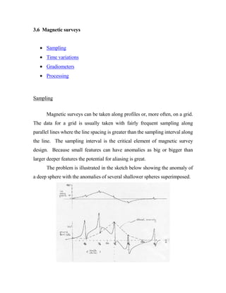
The problem is illustrated in the sketch below showing the anomaly of
a deep sphere with the anomalies of several shallower spheres superimposed.

2. If the sampling interval ∆x is too large, as shown, the anomaly that is
recorded (dashed line) is incorrect. It has been aliased. What has been
recorded does not represent the true anomaly and nothing can be done to
correct the mistake short of redoing the survey. Basically the anomaly must
be sampled with an interval adequate to represent the shortest significant
spatial variation. This can place a severe cost burden on a survey. An
interval of 5 m might be perfectly adequate to map a 40 nT anomaly of a
feature at a depth of 10 m or more but if the surface overburden layer is
scattered with magnetite rich stones which have anomalies of 10 to 100 nT,
then the whole survey has to be made with an interval of 0.5 m. Not
economically reasonable.
A practical solution to this problem is to raise the magnetometer a
distance h above the ground as shown in the above sketch. The amplitudes of
anomalies fall off as the inverse cube of the distance. In raising the
magnetometer from 1 to 2 meters from a shallow target the original anomaly,
which was say 40 nT, is reduced by a factor of 8 to 5 nT. The 40 nT anomaly
from a target 10 m deep is reduced in this process by only about 50 percent
or to about 20 nT. Aliasing at this height is not as much of a problem. The
shallow features only contribute errors on the order of 5 nT. Raising the
magnetometer another meter reduces the shallow anomalies to about 1.5 nT.
Before beginning any survey in a new area it is important to run a few
short lines with a small sample interval to determine the spatial variability of
the fields. Further, while surveying if sudden large changes are noted it is
important to stop, back up, and resample at a closer interval if necessary.
The advantages of getting the magnetometer away from shallow
magnetic anomalies is the principle reason for doing magnetic surveys from
the air. Airborne magnetic surveys have become an indispensable part of

3. mineral exploration and geological mapping projects. Most of the U.S. and
Canada have been surveyed, as well as large parts of the developing world
with mineral and petroleum potential.
Time variations
Time variations must be removed if they are comparable to the
anticipated anomaly and if the duration of that part of the survey covering the
anomaly is comparable to the period of the time variation to be corrected.
Thus, if the survey for the anomaly of a buried steel tank is to be completed in
an hour and the anticipated anomaly is of order 500 nT, the time variation
expected might be on the order of 10 nT and so could be neglected. On the
other hand a magnetic survey over a large area for alluvial magnetite sands
under a thick cover might take all day and the anticipated anomalies might be
100 nT or less. In this case the time variations would be on the order of 30 nT
and they would have to be removed.
There are two main methods used to remove time variations.
i) Return to a base station at a time interval small compared to the
period of the time variation whose amplitude is to be removed. If we have to
have a survey resolution of 1 nT return to a base station every 1000 seconds
may be necessary. This may be reasonable since such high-resolution surveys
are often on a small scale. The corrections are made in airborne surveys by
periodically flying over a base station or by flying cross lines to tie a set of
parallel lines to a set of fixed points.

4. ii) Establish a base station and record the time variations over the
duration of the survey. The time varying fields are uniform, that is they don’t
vary laterally, over 100’s of kilometers. Providing the airborne and ground
magnetometers have a common accurate time base the variations at the base
can simply be subtracted from the airborne readings. This is now common
practice for airborne surveys and it is also used for high accuracy ground
surveys. On the ground the two magnetometers can be physically connected
and the difference in reading is recorded directly.
Gradiometers
The difference scheme discussed in ii) above can be employed using
two magnetometers separated by a small distance ∆x or ∆y in the horizontal
direction or by ∆z in the vertical direction. The difference in field, ∆T,
divided by the spacing is a measure of the derivative or gradient of the field in
the spacing direction. Since the time variations are uniform they are removed
in the gradient operations. In many applications the gradients are as useful as
the field measurements. The gradient operator acts like a high-pass filter - it
accentuates short wavelength anomalies and attenuates broad anomalies from
deep targets. In this sense gradients tend to remove the regional anomalies
from the survey results.

5. Processing
After removing the time variations, magnetic data is usually plotted on
a 2D map and contoured. Once in this format a number of transformations
are possible which enhance certain features in the data. The transformations
are made using a mathematical property of potential fields that allows 2D
maps of any component of a field to be transformed into maps of the same
component at a different elevation (upward or downward continuation) or into
maps of another component, or into maps of the gradient of any component.
Yet another transformation permits the conversion of a map taken at a
given magnetic latitude into a map of what would have been seen if the data
were taken in a vertical inducing field at the magnetic pole. This process is
called reduction to the pole. We have seen that the characteristics of magnetic
anomalies depend greatly on the direction of the inducing field. Reduction to
the pole removes this variable from the maps, putting data taken anywhere on
a common footing for interpretation.