
Recommended
More Related Content
What's hot
What's hot (17)
Viewers also liked
Viewers also liked (20)
Similar to Retrieve pivot table data with INDEX/MATCH
Similar to Retrieve pivot table data with INDEX/MATCH (20)
Retrieve pivot table data with INDEX/MATCH
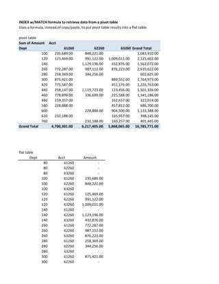
- 1. INDEX w/MATCH formula to retrieve data from a pivot table Uses a formula, instead of copy/paste, to put pivot table results into a flat table. pivot table Sum of Amount Acct Dept 61260 62260 63260 Grand Total 100 235,689.00 848,221.00 1,083,910.00 120 125,469.00 991,122.00 1,009,011.00 2,125,602.00 140 1,129,196.00 432,876.00 1,562,072.00 260 772,287.00 987,112.00 876,223.00 2,635,622.00 280 258,369.00 344,256.00 602,625.00 300 875,421.00 889,552.00 1,764,973.00 420 775,587.00 451,176.00 1,226,763.00 440 258,147.00 1,119,723.00 123,456.00 1,501,326.00 460 778,899.00 336,699.00 225,588.00 1,341,186.00 480 159,357.00 162,657.00 322,014.00 580 228,888.00 457,812.00 686,700.00 600 228,888.00 904,500.00 1,133,388.00 620 232,188.00 165,957.00 398,145.00 760 232,188.00 169,257.00 401,445.00 Grand Total 4,700,301.00 6,217,405.00 5,868,065.00 16,785,771.00 flat table Dept Acct Amount 80 61260 - 80 62260 - 80 63260 - 100 61260 235,689.00 100 62260 848,221.00 100 63260 - 120 61260 125,469.00 120 62260 991,122.00 120 63260 1,009,011.00 140 61260 - 140 62260 1,129,196.00 140 63260 432,876.00 260 61260 772,287.00 260 62260 987,112.00 260 63260 876,223.00 280 61260 258,369.00 280 62260 344,256.00 280 63260 - 300 61260 875,421.00 300 62260 -
- 2. 300 63260 889,552.00 420 61260 775,587.00 420 62260 - 420 63260 451,176.00 440 61260 258,147.00 440 62260 1,119,723.00 440 63260 123,456.00 450 61260 - 450 62260 - 450 63260 - 460 61260 778,899.00 460 62260 336,699.00 460 63260 225,588.00 480 61260 159,357.00 480 62260 - 480 63260 162,657.00 550 61260 - 550 62260 - 550 63260 - 580 61260 228,888.00 580 62260 - 580 63260 457,812.00 600 61260 - 600 62260 228,888.00 600 63260 904,500.00 620 61260 232,188.00 620 62260 - 620 63260 165,957.00 680 61260 - 680 62260 - 680 63260 - 760 61260 - 760 62260 232,188.00 760 63260 169,257.00 751 61260 - 751 62260 - 751 63260 - 890 61260 - 890 62260 - 890 63260 - 16,785,771.00
- 3. INDEX(array,row_num,column_num) Returns a value from within a table or range. =INDEX(A6:E21,2,3) 848,221.00 MATCH (lookup_value,lookup_array,[match_type]) Returns the relative position of a specified item in a range. Use MATCH function to provide a value for the ROW_NUM or COLUMN_NUM argument of the INDEX function. match_type = -1,0,1 (default is 1) -1: smallest value >= lookup value (descending order) 0: first value that = lookup value (any order) 1: largest value <= lookup value (ascending order) =MATCH(A7,$A$6:$A$21,0) 2 =MATCH(C6,$A$6:$E$6,0) 3 Test area: change entries in highlighted area. Note: the second formula returns 0 instead of #N/A. 80 61260 #N/A 100 62260 848,221.00
- 4. Dept Acct Amount 100 61260 $ 112,233.00 100 61260 $ 123,456.00 100 62260 $ 369,258.00 100 62260 $ 478,963.00 120 61260 $ 125,469.00 120 62260 $ 991,122.00 120 63260 $ 457,812.00 120 63260 $ 551,199.00 140 62260 $ 564,598.00 140 62260 $ 564,598.00 140 63260 $ 321,654.00 140 63260 $ 111,222.00 260 61260 $ 772,287.00 260 62260 $ 987,112.00 260 63260 $ 876,223.00 280 62260 $ 128,769.00 280 61260 $ 258,369.00 280 62260 $ 215,487.00 300 61260 $ 875,421.00 300 63260 $ 321,654.00 300 63260 $ 567,898.00 420 61260 $ 775,587.00 420 63260 $ 115,577.00 420 63260 $ 335,599.00 440 62260 $ 132,069.00 440 61260 $ 258,147.00 440 62260 $ 987,654.00 440 63260 $ 123,456.00 460 61260 $ 778,899.00 460 62260 $ 336,699.00 460 63260 $ 225,588.00 480 61260 $ 159,357.00 480 63260 $ 162,657.00 580 61260 $ 228,888.00 580 63260 $ 457,812.00 600 62260 $ 228,888.00 600 63260 $ 447,711.00 600 63260 $ 456,789.00 620 63260 $ 165,957.00 620 61260 $ 232,188.00 760 62260 $ 232,188.00 760 63260 $ 169,257.00 $ 16,785,771.00