1. 6 August 2010
Asia Pacific/China
Equity Research
Analysing Chinese Grey
Income
Expert Insights
New study, new findings
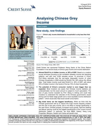
Figure 1: China’s adj. income distributed to households is only less than that
of the US
(US$ tn) (%)
12 80
10 75
2.9
8 70
6 65
4 8.0 60
The Credit Suisse Expert Insights series 1.2 0.9
2 0.4 55
delivers proprietary and independent 2.1 2.1 2.6 0.1
insights leveraging an extensive 0 0.4 50
network of leading experts across all
China (2008) - adj China (2008) - Japan (2008) US (2008) Korea (2008)
sectors and regions.
official
Research Analysts
Wage Other Income % of GDP (RHS)
Vincent Chan
852 21016568 Source: Prof. Wang's Study, NBS, CEIC
vincent.chan@credit-suisse.com
Peggy Chan, CFA Credit Suisse has sponsored Professor Wang Xiaolu of the China Reform
852 2101 6305 Foundation in his second study of China’s grey income and income distribution:
peggy.chan@credit-suisse.com
Gabriel Chan ■ Almost Rmb10 tn in hidden income, or 30% of GDP. Based on a creative
852 2101 6523 survey technique focusing on the correlation between income and spending
gabriel.chan@credit-suisse.com
patterns, and with over 4,000 samples across 19 provinces in China,
Jinsong Du
852 2101 6589 Prof. Wang estimates that the per-capita disposable income of urban
jinsong.du@credit-suisse.com Chinese households in 2008 should be Rmb32,154, 90% above the official
Arndt Ellinghorst data. Total hidden income could total Rmb9.3 tn, 30% of GDP, with about
44 20 7888 0295 63% of hidden income in the hands of the top 10% of urban households.
arndt.ellinghorst@credit-suisse.com
Rogerio Fujimori ■ The potential of China’s consumer market is even bigger than we
44 20 7888 0889 expected. Most investors are aware that Chinese income statistics are
rogerio.fujimori@credit-suisse.com
underestimated, but the exact amount is subject to much speculation. The
Patrick Jnglin
41 44 334 6077
size of grey income revealed by Prof. Wang is striking and could help
patrick.jnglin@credit-suisse.com investors to understand the rationale of the Chinese government’s recent
Cusson Leung strong push for faster wage growth and a more equitable income distribution
852 2101 6621 pattern – which would also help boost overall consumption.
cusson.leung@credit-suisse.com
Kevin Yin ■ Big ticket items are the biggest beneficiary. While we think that the
852 2101 7655 Chinese government will try to reduce this huge income disparity problem
kevin.yin@credit-suisse.com
and the size of the grey income, this is not likely to change significantly in
the near future. Chinese property, European luxury goods, high-end retailing
and Macao gaming could be the biggest beneficiaries of the current income
distribution pattern. In particular, we think BMW, Galaxy, Hang Lung
Properties, Mengniu, Swatch and Vanke will benefit most.
DISCLOSURE APPENDIX CONTAINS ANALYST CERTIFICATIONS AND THE STATUS OF NON-US ANALYSTS. FOR
OTHER IMPORTANT DISCLOSURES, visit www.credit-suisse.com/ researchdisclosures or call +1 (877) 291-2683.
U.S. Disclosure: Credit Suisse does and seeks to do business with companies covered in its research reports. As a result,
investors should be aware that the Firm may have a conflict of interest that could affect the objectivity of this report. Investors
should consider this report as only a single factor in making their investment decision.

2. 6 August 2010
Focus charts and tables
Figure 2: Comparing Wang's study to the official data
(2008) Per-capita disposable Income (Rmb p.a.) % of hidden
Household distribution Official data (1) Wang's study (2) (2)/(1) % income
Bottom 10% 4,754 5,350 113 0.4
10-20% 7,363 7,430 101 0.0
20-40% 10,196 11,970 117 2.3
40-60% 13,984 17,900 128 5.1
60-80% 19,254 27,560 143 10.9
80-90% 26,250 54,900 209 18.8
Top 10% 43,614 139,000 319 62.5
Total 16,885 32,154 190 100.0
Source: NBS Prof. Wang's Study, Credit Suisse estimates
Figure 3: Large share of non-wage income in China Figure 4: Comparing income distribution – China and US
Household disposable Income (% of GDP) (% of total)
80 100
70 90
19.9 80 31.7
60 17.5 47.2 51.9
24.5 70
50 9.9 12.9 60 17.5
50 13.8
40 14.8
40 22.9
30 55.7 30 18.2
52.3 16.0
42.6 47.0 46.2 20 14.7
20 11.2 9.5
10 6.7 9.2 5.4
10 0 4.0
2.9 2.4
0 US Household Income China Official China Disposable
China (2008) - China (2008) Japan (2008) US (2008) Korea (2008) before tax (2007) Disposable Household Household Income -
adj Income (2008) Wang's Study (2008)
Wage Other Income Bottom 20% 20-40% 40-60% 60-80% 80-90% Top 10%
Source: Prof. Wang's Study, NBS, CEIC Source: US Federal Reserve, NBS, Wang's Study
Figure 5: Savings ratio differs a lot between rich and poor Figure 6: GDP and savings ratio adjusted
Sav ings ratio (% of income) 60 52.4 + 4.5% pts 56.0
63.4 + 14.3% pts
70 51.5
60 51.2 50 + 10.3%
50 35.6
40 30.5 40 34.6 38.1
22.7 31.4
30 17.0
20 8.8 30
10
0 20
-10
-20 10
-30 -22.7 0
Rmb7,001 to
Rmb10,001
Rmb17,001
Rmb26,501
Rmb34,000
Rmb75,001
Rmb400,000
Rmb7,000 or
to 400,000
to 17,000
to 26,500
to 34,000
to 75,000
GDP (Rmb tn) Household Sav ings National Sav ings Ration
10,000
below
Over
Ratio (%) (%)
(Annual Disposable Income) Official Adjusted
Source: Prof. Wang's Study Source: Prof. Wang's Study, NBS, Credit Suisse estimates
Analysing Chinese Grey Income 2

3. 6 August 2010
Introduction
Credit Suisse, along with China Society of Economic Reform, has sponsored Prof. Wang Prof. Wang’s second study
Xiaolu of the China Reform Foundation, in his second study on China’s grey income and on China’s grey income and
income distribution. For details on the first study, please refer to Analysing Chinese Grey income distribution
Income, published by Credit Suisse on 3 March 2008.
The recent survey, undertaken in late 2009 (using 2008 data), covers 19 provinces, Sample size of this survey
64 cities and 14 counties, with a total sample size of 4,909. After removing 714 samples was significantly higher at
with either sample quality problems or with negative income in 2008 (for example, due to a 4,195
loss-making family business), the effective sample size is 4,195. This sample size is
significantly larger than the first survey in 2005-06, in which urban residents in
27 provinces, including 49 cities and 14 counties, were surveyed. Some 2,147
questionnaires were returned with 2,054 accepted after verification.
The methodology of the current survey is similar to that of the first. The purpose is to try to The survey aims to
correct the understatement of income in the official household survey by the National reconcile the income that we
Bureau of Statistics (NBS). Basically, the study assumes that while respondents think was understated by
understate their income during the survey of NBS (for reasons like worrying that such NBS
information will be passed to tax authorities, etc.), they have no incentive to understate
total spending, particularly the percentage of food consumption to total spending (the
Engel’s coefficient). Based on this assumption, the survey employs interviewers’ questions
about income, spending and food consumption from the 4,000 plus respondents whom
they know personally. The assumption is that as the interviewer knows the respondent
personally, the respondent will feel more comfortable and willing to disclose their “true”
income. Then, based on the corresponding Engel’s coefficient, the income data collected
in this study is used as a reference, combined with some econometric adjustments, to
adjust the data reported in the official household survey by NBS.
‘Actual’ income could be much higher
Compared to official data, per-capita incomes in Prof. Wang’s Study for every household
group are higher than official data. The average difference is a startling 90%! However, it
is clear that the gap is much larger for the top 20% of income households, while the gap
between Wang’s study and official data is very limited for low-income households.
Figure 7: Comparing Wang's study to the official data
Household income revealed
(2008) Per-capita disposable Income (Rmb p.a.)
by Prof. Wang’s study is on
Household distribution Official data (1) Wang's study (2) (2)/(1) %
average 90% higher than
Bottom 10% 4,754 5,350 113
the official data
10-20% 7,363 7,430 101
20-40% 10,196 11,970 117
40-60% 13,984 17,900 128
60-80% 19,254 27,560 143
80-90% 26,250 54,900 209
Top 10% 43,614 139,000 319
Total 16,885 32,154 190
Source: NBS Prof. Wang's Study, Credit Suisse estimates
Compared to the first study in 2006 (using 2005 data), the 2009 study (on 2008 data) Income gap is widening and
revealed some very interesting differences: 1) the gap between the average income of the second top 10% of
Wang’s study versus official data has risen from 77.7% to 90.4%, i.e. the problem of income households is also
hidden income in these three years is rising; 2) while the income gap between Wang’s starting to benefit from
study and official data has been roughly the same for the top 10% of households, it has hidden income
increased substantially for the other 80-90% of households, from 38.7% to 109.1%. This
means that the second 10% of richest households is starting to “benefit” significantly from
hidden income. If we assume (as Prof. Wang does) that Chinese grey incomes mainly
come from illegal or quasi-illegal income, then this is worrying, as such income is now
Analysing Chinese Grey Income 3

4. 6 August 2010
becoming more widespread among a wider group of the population; 3) most of the hidden
income is concentrated in the top 20% of households. Together, they account for 81.3% of
hidden income, within which the top 10% of households accounts for 62.5%.
Figure 8: Comparing the 2005 and 2008 data from Wang's study
Over 80% of grey income
Wang's study/Official data (%) % of income
comes from the top 20% of
Household distribution 2005 2008
households
Bottom 10% 99.1 112.5 0.4
10-20% 101.8 100.9 0.0
20-40% 106.9 117.4 2.3
40-60% 114.0 128.0 5.1
60-80% 130.6 143.1 10.9
80-90% 138.7 209.1 18.8
Top 10% 337.6 318.7 62.5
Total 177.7 190.4 100.0
Source: Prof. Wang's Study, Credit Suisse estimates
If we assume that there is no underestimation of rural income, then Prof. Wang’s study of Household disposable
2005 and 2008 data reveals the following trends: 1) growth of total disposable incomes income is roughly growing
during this period is roughly equal to GDP, instead of lagging it as official data suggests; 2) as fast as GDP
the growth of hidden incomes, however, is much faster than normal income; therefore, as
a percentage of GDP, hidden income increased from 26.5% to 29.5%, and this contributes
to the widened income gap in China.
Figure 9: Income changes between 2005 and 2008
Grey income is growing at a
2005 2008 Change (%)
much faster rate
Per-capita urban disposable income (Rmb, official data) 11,100 16,885 52.1
Per-capita urban disposable income (Rmb, Wang's study) 19,730 32,154 63.0
Urban population (mn) 562 607 7.9
Per-capita rural net income (Rmb) 3,537 5,171 46.2
Rural population (mn) 745 721 -3.2
Total disposable income (Rmb bn, official data) 8,876 13,974 57.4
Total disposable income (Rmb bn, Wang's study) 13,727 23,237 69.3
Estimated hidden income (Rmb bn) 4,851 9,263 91.0
GDP (Rmb bn) 18,322 31,405 71.4
Total disposable income (% of GDP, official data) 48.4 44.5 -4.0
Total disposable income (% of GDP, Wang's study)* 74.9 74.0 -0.9
Estimated hidden Income (% of GDP)* 26.5 29.5 3.0
Source: Prof. Wang's Study, NBS
In this new report, Prof. Wang distinguishes between the two concepts of “hidden income”
and “grey income”. “Hidden income” is defined as the difference between the total
household disposable income estimated from his study (Rmb23.2 tn in 2008) and official
household disposable income from the NBS household income survey (Rmb14.0 tn in
2008), which amounted to Rmb9.3 tn in 2008. “Grey income” is defined as the difference
between Wang’s estimated household disposable income (Rmb23.2 tn in 2008) and
household disposable income (Rmb 17.9 tn in 2008) revealed in the flow of funds (FOF)
accounts estimated from the Economic Census (data collected from enterprises),
amounting to Rmb5.4 tn in 2008.
Re-estimating the distribution to households
Based on these new results, Prof. Wang has re-estimated the wage and non-wage income GDP distributed to Chinese
for Chinese households, with the estimated grey income added to non-wage income while households is much higher if
wage income remains unchanged. Also, it is assumed that 60% of grey income is not grey income is included
captured in the official national account statistics, so is added back to the national income
and GDP data. Comparing the results of China with other countries, the impact of this grey
income adjustment is very large and clear. Before the adjustment, the share of GDP
Analysing Chinese Grey Income 4

5. 6 August 2010
distributed to households in China is very low compared to developed world economies
such as the US and Japan, particularly for non-wage income. However, if the grey income
is included, the picture changes drastically: 1) distribution to households in China is only
slightly smaller than that of the US and Japan, and well above Korea’s; and 2) non-wage
income, instead of being very small as the official data suggests, was actually very large –
even bigger than a capitalistic market economy, such as the US.
Figure 10: Large share of non-wage income in China
Portion of non-wage
Household disposable Income (% of GDP) income/GDP in China
80 (24.5%) is higher than that
70
in the US (20%)
19.9
60 17.5
24.5 12.9
50 9.9
40
30 55.7
47.0 52.3
42.6 46.2
20
10
0
China (2008) - adj China (2008) Japan (2008) US (2008) Korea (2008)
Wage Other Income
Source: Prof. Wang's Study, NBS, CEIC
We have compared the distribution of per-capita income between US and Chinese
households (based separately on the official NBS household income survey data and
estimates from Wang’s study), assuming that the urban population is roughly equal to the
rural population in China and there is no underestimation of rural personal incomes.
Estimates from the official survey show Chinese household income to be much more
evenly distributed than for the US, while income distribution based on Wang’s study shows
that the distribution pattern of Chinese cities is actually rather similar to that of the entire
US society. This seems to fit better, with income distribution in China slightly more uneven
than in the US and in fact seems more consistent with what we observed.
One very interesting observation to argue for the highly uneven income distribution in Strong buying power of the
China is reflected in the strong buying power of its richest people. For example, according rich Chinese
to our analysts, despite their strong position in the China market, China only accounts for
3% and 5% of sales for Volkswagen and Pepsi, respectively. In contrast, Greater China
(mostly mainland China, as they are also major buyers of such items in Hong Kong)
accounted for 10%, 20% and 28% of sales by LVMH, Richemont and Swatch Group
respectively – all major luxury goods companies. See also our China Consumer Survey –
Consumption Jump, published on 8 January 2010.
Analysing Chinese Grey Income 5

6. 6 August 2010
Figure 11: Comparing income distribution – China and the US Based on Wang’s study,
China’s income distribution
(% of total)
is not as evenly distributed
100 as official data suggests
90
31.7
80
47.2 51.9
70
60 17.5
50
13.8
40 22.9 14.8
30 18.2
16.0
20 14.7
11.2 9.5
10 6.7 9.2 5.4
0 4.0 2.4
2.9
US Household Income before tax China Official Disposable Household China Disposable Household Income
(2007) Income (2008) - Wang's Study (2008)
Bottom 20% 20-40% 40-60% 60-80% 80-90% Top 10%
Source: US Federal Reserve, NBS, Wang's Study, Credit Suisse estimates
The implication of this analysis is that overall income distribution in China is comparable to More equally distributed
other countries. But with a large portion derived from grey income, it is concentrated in a income would help to boost
small group of people with a very high savings ratio. So, if income distribution becomes consumption
more equitable, it would help boost the consumer market. Based on the data in Prof.
Wang’s survey, for those respondents earning less than Rmb7,000 per capita in 2008,
they spend more than their income (i.e. negative savings), while those earning Rmb7,001-
10,000 had a savings ratio of only 8.8%. In contrast, the highest income group earning
over Rmb400,000 had a savings ratio much higher at 63.4%.
Figure 12: Savings ratio diverges significantly between rich and poor
The highest income group
Sav ings ratio (% of income) saves 63.4% of their income
70 63.4
whereas the lowest income
60 51.2
group spends more than
50
35.6 they earn (a negative
40 30.5
22.7 savings rate of -22.7%)
30 17.0
20 8.8
10
0
-10
-20
-30 -22.7
Rmb7,001 to
Rmb7,000 or
Rmb10,001
Rmb17,001
Rmb26,501
Rmb34,000
Rmb75,001
Rmb400,000
to 400,000
to 17,000
to 26,500
to 34,000
to 75,000
10,000
below
Over
(Annual Disposable Income)
Source: Prof. Wang's Study
Impact on Chinese consumption
The existence of such large grey income also means that the size of the economy will be The actual GDP and
bigger, with the actual savings ratio higher. According to Prof. Wang’s study, household savings ratio should be
disposable income in China should be about Rmb23.2 tn, almost Rmb10 tn higher than higher if we take account of
the level revealed in the NBS household survey. However, the gap is smaller (only the grey income
Rmb5.3 tn) when we compare this to the estimated level of household disposable income,
Analysing Chinese Grey Income 6

7. 6 August 2010
at Rmb17.9 tn, under the Flows of Funds Accounts in China’s National Account Statistics.
If we assume 60% of this gap is due to underestimation of actual GDP/national income,
while 40% is wrongly classified under corporate and government income, then China’s
GDP in 2008 would be Rmb34.6 tn 10% above the official level. Household and national
savings ratios would also increase by 14.3 p.p. and 4.5 p.p., respectively. A larger
economy and higher savings ratio mean that the potential of China’s consumer market
(including demand for consumer-related commodities like oil and agricultural products)
could be even bigger.
Figure 13: GDP and savings ratio adjusted
60 52.4 + 4.5% pts 56.0
+ 14.3% pts
51.5
50 + 10.3%
40 34.6 38.1
31.4
30
20
10
0
GDP (Rmb tn) Household Sav ings Ratio (%) National Sav ings Ration (%)
Official Adjusted
Source: Prof. Wang's Study, NBS, Credit Suisse estimates
Indeed, as we argued in China Market Strategy – A Brave New World, published on Based on our assumptions,
14 June 2010, if we assume a 1 p.p. increase in the urbanisation ratio p.a. and wages the consumption to GDP
increase 2 p.p. faster than GDP growth (a possible consequence of the government’s ratio would increase 6.3%
efforts in income distribution reform), then based on the NBS household survey data, between 2009 and 2015
household consumption as a percentage of GDP increases 6.3 p.p. between 2009 and
2015. While most investors and the Chinese government expect Chinese consumption to
become a more important driver of economic growth, we do not think anyone has built in
such expectations in their growth model for China. This, therefore, could be a real surprise
to the market.
Figure 14: Key assumptions of the consumption model
2000-09 2010E 2011-15E
Urbanisation ratio (p.p. change p.a.) 1.2 1.0 1.0
Nominal GDP growth (% change p.a.) 14.6 15.0 11.0
Urban wage (% change p.a.) 12.0 17.0 13.0
Urban non-wage income (% change p.a.) 15.3 15.0 11.0
Rural income (% change p.a.) 9.7 15.0 11.0
2000 2009 2015E
Urban consumption as % of income (avg.) 79.4 65.0 68.0
Rural consumption as % of income (avg.) 74.1 77.5 77.5
Source: CEIC, Credit Suisse estimates
Analysing Chinese Grey Income 7

8. 6 August 2010
Figure 15: Consumption boost
1995 2000 2005 2009 2010E 2015E
Total population (mn) 1,211 1,267 1,308 1,335 1,341 1,375
% change 4.6 3.2 2.1 0.5 2.5
Urban population (mn) 352 459 562 622 638 723
% of total 29.0 36.2 43.0 46.6 47.6 52.6
GDP (Rmb bn) 6,079 9,921 18,494 33,535 38,566 64,985
% change 63.2 86.4 81.3 15.0 68.5
Urban wage per capita (Rmb) 3,390 4,481 7,798 12,382 14,487 26,691
% change 32.2 74.0 58.8 17.0 84.2
Total payroll – urban (Rmb bn) 1,192 2,057 4,383 7,700 9,248 19,305
% change 72.5 113.1 75.7 20.1 108.7
% of GDP 19.6 20.7 23.7 23.0 24.0 29.7
Urban non-wage income (Rmb bn) 313 833 1,980 4,027 4,754 9,076
% change 166.6 137.6 103.3 18.1 90.9
Urban household income (Rmb bn) 1,505 2,890 6,364 11,727 14,003 28,382
% change 92.0 120.2 84.3 19.4 102.7
% of GDP 24.8 29.1 34.4 35.0 36.3 43.7
Urban consumption per capita (Rmb) 3,538 4,998 7,943 12,265 14,375 26,698
% of income 82.7 79.4 70.2 65.0 65.5 68.0
Urban consumption (Rmb bn) 1,244 2,019 4,465 7,627 9,177 19,310
% change 62.3 121.1 70.8 20.3 110.4
% of GDP 20.5 20.4 24.1 22.7 23.8 29.7
Rural net income per capita (Rmb) 1,578 2,253 3,255 5,153 5,926 9,986
% change 42.8 44.4 58.3 15.0 68.5
Rural consumption per capita (Rmb) 1,310 1,577 2,555 3,994 4,593 7,739
% of income 83.1 70.0 78.5 77.5 77.5 77.5
Rural consumption (Rmb bn) 1,126 1,350 1,905 2,847 3,229 5,046
% change 19.9 41.1 49.5 13.4 56.3
% of GDP 18.5 13.6 10.3 8.5 8.4 7.8
Total consumption (Rmb bn) 2,371 3,369 6,370 10,474 12,406 24,356
% change 42.1 89.0 64.4 18.4 96.3
% of GDP 39.0 34.0 34.4 31.2 32.2 37.5
Source: CEIC, Credit Suisse estimates
Income inequality could cause social issues
Another issue concerning the large amount of grey income is the social stability issue. Grey income worsens the
According to various estimates, including that of the United Nations, the Gini coefficient (a inequality that could cause
measurement of income inequality) of China, based on the official data, is already social instability
between 0.45-0.5, roughly equal to the US but higher than other developed countries such
as Japan and in Europe. If the effect of grey income is included, China’s Gini coefficient
would be even higher, similar to that of South American countries, but hopefully still better
than the African continent.
Analysing Chinese Grey Income 8

9. 6 August 2010
Figure 16: Gini coefficient based on official data
Source: Wikipedia
Against this background, from a few years ago, it is clear that the Chinese government has The government is already
started to adopt policies trying to address social inequality, such as enacting the Labour taking action to address this
Contract Law in 2008. Also, the government as well as the Chinese media are also taking social inequality
a rather open (to a certain extent, supportive) attitude towards the labour unrest in
Guangdong during the industrial disputes earlier this year, which has driven industrial
wages to rise across China. Such attitudes to allow labour costs to rise in China have not
been seen during the earlier years of Chinese economic reform. Also, it is widely reported
in the Chinese media that the Chinese government will announce a new reform initiative
this year called ‘Income Distribution Reform’, probably around the time of the
announcement of the 12th Five-Year Plan (for 2011-15). The purpose of this reform is to try
to address unequal income distribution in China, and there are some news reports (such
as on Sina.com) saying that the government is targeting to double the wages of
manufacturing workers in next five years.
Few details suggest how the government is planning to achieve this target, but we expect Wages to have to be raised
the following action to be taken:
(1) The government will take the initiative to raise wages in state-owned enterprises
(SOEs), which, in turn, should drive wage growth in the non-state sector;
(2) Individual provincial/city governments will continue raising minimum wages across
China; and
(3) The role of collective bargaining will rise. The government is likely to strengthen the
function of the All-China Federation of Trade Unions (ACFTU). Instead of taking a
rather passive position as in the past few decades, this government-sponsored trade
union body (headed by the Vice Chairman of the National People’s Congress (NPC)
who is also a member of the Politburo in the Chinese Communist Party) is likely to
take a more detailed role in promoting workers’ rights and wage negotiations.
This reform deserves a lot of attention from investors, in our opinion. On the one hand, if it Higher wages benefit the
is successful in boosting the wages of workers, this would help develop the Chinese consumer market, but are
consumer market, as well as reduce the risk of social instability due to social inequality. bad for employers
However, based on economics history, active government involvement in wage
negotiations usually results in reducing the flexibility of the labour market, which may not
be positive when China faces its next major economic downturn similar to in the late
Analysing Chinese Grey Income 9

10. 6 August 2010
1990s. One way or another, this reform could affect the investment environment of China
stocks significantly.
Sector and stock beneficiaries
In this report, we also highlight a number of sectors/stocks which we think are major
beneficiaries of this widespread grey income phenomenon in China. They include China
property, European luxury goods, Macau gaming and some Hong Kong property investors
with large exposure to the high-end retail space in Hong Kong. Stocks included in this
report are: BMW, COLI, Galaxy, Hang Lung Properties, KWG, LVMH, Mengniu,
Richemont, Swatch and China Vanke.
Analysing Chinese Grey Income 10

11. 6 August 2010
The translated version of Professor
Wang Xiaolu's report on China’s
grey income and income
distribution (2nd survey study)
Analysing Chinese Grey Income 11

12. 6 August 2010
Analysing Chinese grey income
Between 2005 and 2006, the National Economic Research Institute of the China Reform
Foundation conducted an income and consumption survey of urban residents in different
cities of China. In 2007, the deputy director of the institute, Professor Wang Xiaolu,
published a study report entitled Grey Income & Income Inequality in China, based on the
survey. Professor Wang thinks that the disguised incomes, totalling Rmb4.8 tn of the
disposable income of urban residents in 2005, which were not reflected in the statistics of
residential income (“hidden income”), mainly belong to the high income class. A correction
of the income data by including the hidden income shows that the gap between the top
10% of household incomes and the bottom 10% in urban areas widens to 31 times rather
than the originally calculated 9x, while the gap between the top 10% of household incomes
and the bottom 10% household incomes on a nationwide basis, reaches 55 times instead
of the original 21. These figures mean that the income inequality problem is more severe
than what we knew before.
The report also makes estimations of residential incomes – mainly those of higher income Other than analysing
residents – from different perspectives according to data concerning family ownership of Chinese grey income, the
cars, sales of commercial housing, numbers of overseas travels per person and bank report also estimate
savings. The results of the above estimations were cross validated to prove their accuracy. residential incomes from
Meanwhile, through a primary analysis of the sources of grey income, the author argues different perspective
that the phenomenon is caused by a loophole in the system and therefore demands an
urgent system reform to solve the imbalance.
To what degree are the methods and results of the above estimations credible? What sort The second report was
of changes has occurred to national income distribution in all these years? To answer published in 2009 and has
these questions, we conducted another survey of urban residents’ incomes and expenses new study analysis
in 2009 (data from the full year of 2008), and made a new study and analysis based on it.
The following report states the scope of this survey, the methodology and analysis, and
final results, as well as further analysing the income equality issue and its relevant
countermeasures.
Part One of the report informs us about the methodology of the survey and the distribution There are six parts to the
of the survey samples. Part Two states the methodology of analysis and the result of the report
analysis. Part Three estimates the genuine standard of the disposable incomes of urban
residents and the actual income gap. Part Four is a further analysis of the sources of grey
income. Part Five analyses the influence of grey income upon the structure of national
income distribution. Part Six is the conclusion of the report.
Analysing Chinese Grey Income 12

13. 6 August 2010
1) Sampling methodology and
sample distribution
How to obtain genuine data
We contend that the present statistics on residential incomes have major distortions, Random sampling was used
especially in the part concerning the disposable income of high-income residents in urban to determine resident
areas. These distortions do not lie within the methodology of the survey or calculation. samples
Currently, samples of urban and rural residents are determined by random sampling. There
is nothing wrong with this method in itself, but attention should be paid to the following:
1) Current random sampling is based on the principle of voluntary participation. A
considerable proportion of higher income residents, however, is unwilling to do the
survey. The samples, therefore, have to be replaced by someone else’s, and those of
higher income residents are left out.
2) Among those higher income residents in the sampling, many were reluctant to provide
genuine income information. They tend to report truthfully their salaries, but are
relatively untruthful about other income, especially those considerable hidden “grey
incomes” from unidentifiable sources. This part of income is definitely impossible to
reflect in the survey data.
For these reasons, deviations of data tend to occur and the survey fails to reflect the Deviations exist but there is
genuine income distribution of residents. With current samples and methodology, there no easy solution
can be no easy solution to this. A new way of studying is required. For this reason, the first
and foremost purpose of our study is to obtain genuine data about residential income. In
the 2005-06 survey, we drew on the methods of sociology and asked our professional staff
to investigate the family incomes and expenses of their relatives, friends, colleagues and
neighbours. We also took certain supplementary measures to ensure the authenticity of
the data. It proves that this method worked and we did have data of relatively higher
accountability.
In the 2009 survey, we adopted the same method, but implemented stricter quality control
measures and increased the quantity of samples. It is worthwhile to know that our method
is different from that of random sampling and therefore the data cannot be used directly to
calculate the general distribution of urban residential income. A detailed introduction of our
calculation methods is given in Part Two of this report. In this part, we focus on the
explanation of our survey methodology and distribution of samples.
Before the survey, we organised for our staff at various locations training on questionnaire Questionnaire and
and survey methodology. To eliminate the interviewees’ doubts, the questionnaires were interviewee training
anonymous and the interviewees were assured of the research purpose of the survey as
well as confidentiality of their personal data. We also took measures to lower the
sensitivity of the survey to ensure data authenticity. For instance, we emphasised that our
purpose is to study consumption structure instead of income levels. The questionnaire is
designed to inquire about consumption issues before the income issues, and to inquire
about different divisions before the income and consumption total. As for the sources of
incomes, the questionnaire only asked the interviewees to choose among simple divisions
of income, such as salary, part-time and service revenue, entity-business, financial
investment, property, intellectual property, transferred income and other incomes. After the
survey, the staff were required to report about their relationship with the interviewee and
their personal estimation about the accountability of the survey result (including possible
deviations and degree of deviation) as references for the questionnaires.
After the completion of the survey, we made a thorough quality inspection of the Quality inspection post
questionnaires. Apart from verification of information integration and survey locations, we survey completion
also designed a set of inspection procedures to examine the rationality of the logic for
Analysing Chinese Grey Income 13

14. 6 August 2010
each question and check whether the relationship of income and expenditure data in the
sample is reasonable or not. We then exclude those disqualified questionnaires (including
those with much information left out, altered, containing abnormal or illogical information
and were impossible for us to identify whether correct, and those from non-urban
residents) and questionnaires whose information authenticity was doubtful.
The distribution of survey samples
This survey was conducted in 64 cities of different scale in 19 provinces (including cities
under direct management of the central government), as well as 14 counties and organic
towns.
The provinces (including cities under direct management of the central government) are The survey is conducted in
Beijing, Shanghai, Shandong, Jiangsu, Zhejiang, Guangdong, Shanxi, Henan, Hubei, 64 cities from 19 provinces
Anhui, Jiangxi, Liaoning, Heilongjiang, Sichuan, Chongqing, Yunnan, Shanxi, Gansu and
Qinghai. The cities are Beijing, Shanghai, Jinan, Nanjing, Hangzhou, Guangzhou, Taiyuan,
Zhengzhou, Wuhan, Hefei, Nanchang, Shenyang, Harbin, Chengdu, Chongqing, Kunming,
Xi’an, Lanzhou, Xining, Shenzhen, Qingdao, Suzhou, Datong, Anshan, Wushun, Tsitsihar,
Daqing, Xuzhou, Yangzhou, Fuyang(in Anhui Province), Wuhu, Lu’an, Rizhao, Xiangfan,
Yichang, Dongwan, Zhongshan, Mianyang, Xinzhou, Kaifeng, Sanmenxia, Zhumadian,
Xiaogan, Yidu, Pizhou, Fuyang(in Zhejiang Province), Jinhua, Shaoxing, Shaoguan,
Chaohu, Chuzhou, Ganzhou, Ji’an, Jindezhen, Jiujiang, Dandong, Tieling, Mudanjiang,
Xichang, Xianyang, Baiyin, Jiayuguan, Tianshui and Yuxi. Among these, 21 are cities
under direct management of the central government, provincial capitals or sub-provincial
cities, 43 are small prefecture cities and county-level cities. In this way, a relatively
balanced distribution was kept among cities of different scales.
Counties and organic towns include Fanzhi County in Shanxi Province, Pei County in 14 counties and organic
Jiangsu Province, Xiangshan County in Zhejiang Province, Pingyuan County and Qihe towns
County in Shandong Province, Hua County in Henan Province, Dawu County in Hubei
Province, Zhijiang County, Kai County and Zhong County in Chongqing City, Liquan
County in Xianyang City of Shanxi Province, Gaolan County and Jingchuan County in
Gansu Province and Minhe County in Qinghai Province. The geographical distribution of
these counties was also relatively balanced.
This survey has chosen a large amount of cities with a relatively scattered distribution of
samples, mainly for two reasons. First, if we choose too many samples in a city, we cannot
ensure that our staff are all familiar with the respondents – which is a prerequisite of the
survey. Second, as the samples are from relatively many cities, they can be more
representative of the national economic situation.
Our methodology has its own shortcomings. A major problem of the survey is that the The shortcomings of our
survey is non-recurring, and all the data about the income and consumption of the methodology
interviewed families are provided by the interviewee according to their memory (though we
have excluded those family members who are unfamiliar with their family incomes and
consumption).Compared with surveys requiring respondents to record their income and
expenditure, this might cause greater data error. However, requiring respondents to record
their information over a extended period of time is more costly, time-consuming and
difficult, and more prone to systematic distortion due to sensitivity of the survey questions.
Data errors in the non-recurring survey, due to inaccurate memory, are mostly random
instead of systematic. In the sense that the result is calculated by taking the average,
random errors should offset each other and decrease, while systematic distortions cannot
be offset. In view of our research purpose and conditions, we must therefore adopt non-
recurring means for the survey.
This survey included 4,909 sample families. After a strict quality inspection, 689 The effective sample size is
disqualified questionnaires were deleted, 25 negative income samples were excluded from 4,195.
the analysis (as the analysis showed that most of these families were not low in income
Analysing Chinese Grey Income 14

15. 6 August 2010
most of the time. Negative income families were mainly suffering from a temporary
operational deficit). The effective sample size therefore is 4,195.
Figure 17 gives us information about the regional distribution of all samples and effective The samples are generally
samples, the scales of the cities, the age and household registration of the respondents, evenly distributed but we
the education level of the maximum income earners of the sample families, the distribution have intentionally increased
of per-capita disposable incomes of the interviewed family and others. The samples are samples of higher income
generally evenly distributed in different regions and cities of different scales, and among group in urban areas
interviewees of various ages and education levels. However, it seems that the survey
sample is skewed to people living in larger cities, with better education, owning their
business or working in white collar positions. This is done for a reason. According to the
results of the 2007 report, the statistical distortion of urban residential incomes mainly
occurs with higher income residents. In order to ensure enough samples of higher income
residents for analysis, we intentionally increased the number of samples for this group of
people. In this way, we could make sure that the difference of distribution has the least
impact on the estimation of per-capita income distribution of national urban residents.
Analysing Chinese Grey Income 15

16. 6 August 2010
Figure 17: Sample distribution by different groups
Sample Effective
Total distribution Sample Proportion
Samples (%) Distribution (%)
1. Geological location
Eastern region 1,863 37.95 1563 37.26
Middle and Northeast 1,848 37.65 1605 38.26
Western region 1,198 24.40 1027 24.48
Total 4,909 100.00 4195 100.00
2. Scale of the cities
Cities with more than 2 mn in population 2,495 50.83 2,083 49.65
Cities with 1 to 2 mn in population 915 18.64 789 18.81
Cities with less than 1 mn in population 995 20.27 889 21.19
Counties and organic towns 504 10.27 434 10.35
Total 4,909 100.00 4,195 100.00
3. Age of the interviewees
20-29 1,647 33.55 1,411 33.64
30-39 1,383 28.17 1,196 28.51
40-49 1,236 25.18 1,062 25.32
50-59 520 10.59 425 10.13
60 and above 123 2.51 101 2.41
Total 4,909 100.00 4,195 100.00
4. Registration of the interviewees
Local urban citizens 4,457 90.79 3,808 90.77
Non-local urban citizens 276 5.62 234 5.58
Non-local rural citizens 156 3.18 138 3.29
Forget to answer 20 0.41 15 0.36
Total 4,909 100.00 4,195 100.00
5. Highest educational level in the family
Elementary school and below 165 3.36 136 3.24
Junior middle school 970 19.76 832 19.83
Senior middle school(including equivalency) 1,833 37.34 1,565 37.31
Junior college and undergraduate 1,822 37.12 1,569 37.40
Post-graduate and PhD 82 1.67 74 1.76
Forget to answer or indefinable 37 0.75 19 0.45
Total 4,909 100.00 4,195 100.00
6. Highest income profession of the family
General technician 396 8.07 353 8.41
Intermediate and advanced technicians 262 5.34 227 5.41
Other professionals(science, education, culture and health) 339 6.91 302 7.20
Cadre of the Party, government offices, army and institutions 193 3.93 165 3.93
Advanced cadre of the Party, government offices, army and institutions 52 1.06 47 1.12
Staff of enterprises, govt. organizations and communities 561 11.43 483 11.51
Middle-level manager of enterprises and govt. organisations 327 6.66 268 6.39
Service industry 317 6.46 277 6.60
Worker 659 13.42 562 13.40
Personal business, freelancer 1,008 20.53 853 20.33
Owner, partner, shareholder of private enterprises 317 6.46 277 6.60
Other professions 73 1.49 66 1.57
Students, post-graduates 20 0.41 17 0.41
The jobless (including the retired and the resigned) 349 7.11 278 6.63
Forget to answer or indefinable 36 0.73 20 0.48
Total 4,909 100.00 4,195 100.00
Note: the scale of the city is measured by its permanent urban population. Source: Survey Sample Data.
Analysing Chinese Grey Income 16

17. 6 August 2010
2) Analysis methodology and
results
Engel’s coefficient
First, we conducted the survey of urban residential incomes not for the direct estimation of Engel’s coefficient
general income distribution of urban residents, but for the estimation of the relationship (proportion of food
between income level and the consumption pattern, based on genuine data with which expenses in consumption
there is no underestimation of income. Such information is then used later to “adjust” the outlay) is an index closely
income data of the official household survey of the NBS. One of the key variable is the connected with the income
Engel’s coefficient, which refers to the proportion of food expenses in consumption outlay. level
Engel’s coefficient is an index closely connected with income level. It has been recognised
in the economic profession that the decline of Engel’s coefficient usually correlates with
the rise of income levels. After their basic needs for food and clothing are satisfied,
residents gradually turn to other needs, such as the need for transportation and
communication, luxuries, as well as higher level demand for education and cultural
entertainment. With higher income levels, their incremental food expenditure declines,
resulting in a lower level of food consumption to total consumption expenditure.
Based on this principle, we can choose a relatively trustful and typical survey sample to Engel’s coefficient can be
calculate the Engel’s coefficient and per-capita disposable income of the family, and use used to estimate per capita
statistical theory or econometrics studies to find their statistical relationship. With this above income
correlation, we can examine any set of residential income statistics. In other words, we need
only a set of relatively credible Engel’s coefficient to estimate the genuine income level per
capita. Therefore, based on the Engel’s coefficients of group urban residents by NBS, we
can estimate the average income levels of these groups and compare the result with the
published income statistics. We can notice whether or not a systematic distortion exists and
how large the distortion can be. We call this kind of method “Engel’s Ratio Method”.
Of course, the prerequisite of this method is to ensure the authenticity of the Engel’s Deviations in calculating
coefficients in group census samples. If we are likely to encounter such a problem, i.e. if the Engel’s coefficient are
income level statistics of some groups have systematic deviations, would the relevant generally acceptable
Engel’s coefficients have the same systematic deviation? Actually, while there might be
some deviation in income data (underestimated, for instance), the consumption expenses
are very likely to involve certain deviations too. As long as both deviations are of the same
direction and maintain relatively the same proportion in the statistical sense, then the
average group of Engel’s coefficients is still basically credible. We can continue to use this
Engel’s coefficient to estimate genuine income levels. Second, even if consumption
expenses and food expenses have different proportions of deviations, deviations of the
same direction can be offset to a large extent in calculating the Engel’s coefficient to
minimise the error in the final result. Therefore, it can still be used to estimate income levels.
According to the 2007 study, the official income data of the highest income residents had
the greatest distortion and were far lower than their “real” incomes. There were certain
underestimates about their consumption and food expenses, but not as obvious as the
under-reporting of their incomes. Food expenses, in general, involve less deviation than
the total consumption. This means that the calculated Engel’s coefficient might be slightly
higher and the estimated income level might be slightly lower, yet a large part of the data
deviation can be offset. We have to note, however, that the final result of the income level
might still be a little bit lower than the “real” incomes, to some extent.
Another fact that we need to be aware of is that the Engel’s ratio method used to examine
the statistical data of residents’ incomes can only make corrections upon systematic errors
of the existing samples, without ascertaining the actual quantity of omitted higher income
residents. Therefore, the final result might still underestimate the income levels of higher
income residents to some extent (due to sample omission).
Analysing Chinese Grey Income 17

18. 6 August 2010
In the following part, the author has used two concrete methods to set up the correlation
between Engel’s coefficient and the income level, in an effort to examine residents’ income
data. Both methods belong to the Engel’s ratio method, but are slightly different in terms of
analysis and procedures. For the sake of convenience and distinction, the author
abbreviates “per-capita disposable income” into “per-capita income”, survey samples of
urban resident households by NBS into “official sample”, samples of our survey into “study
samples”, per-capita income from official data into “official income”, and per-capita income
estimated by comparing the parameter of survey samples and official data into “estimated
income”.
Group comparison
First, we calculate the per-capita income and Engel’s coefficients of all survey samples
respectively.
Second, we calculate the group Engel’s coefficient of the official data. The group income
data, issued by the NBS annually, divide the urban resident families into seven groups
according to their per-capita incomes. Among these, the minimum income, low income,
maximum income and high income are further divided into ten equal quantities, with each
group taking 10% of the urban families. The three groups in the middle, namely the lower
middle income, middle income, and upper middle income groups, are further divided into five
equal quantities, with each group comprising 20% of the urban families. The average Engel’s
coefficient of the seven groups can then be calculated. Based on the explanation in the
former chapter, we assume that the Engel’s coefficient of the official sample is correct.
Third, we sort all the effective survey samples according to per-capita income, from the
lowest to the highest. By group comparison method, we mean that samples of lowest
income need to be added until their average Engel’s coefficient equals that of the
“minimum income of the official sample”. This chosen group sample is called “minimum
income group of the survey sample”. This process of grouping does not require
consideration of sample quantities. Then, the same method is used to group the “low
income group of the survey sample”, to make its average Engel’s coefficient equal with the
“low income of the official sample” (the above-mentioned second 10% of urban residents).
This applies for each grouping.
Fourth, we calculate the average per-capita income of each group of the survey samples
respectively. For reasons explained in the previous chapter, we assume that the Engel’s
coefficient of each group has an exclusive correspondence with their income level. In other
words, we can calculate the per-capita income given the Engel’s coefficient of each group
correspondingly.
Finally, we compare the per-capita income of the survey samples with that of the
corresponding official sample and discover the underestimation of income in the official
sample. Figure 18 shows the group distribution of the survey samples and official samples.
We can see from the form that group distribution of survey samples differ from each other
though the same Engel’s coefficient is taken. We can also discover that some survey
samples with the highest per-capita income are left out of the seven groups because their
Engel’s coefficients are even lower. These people have an annual disposable income of
more than Rmb400,000, with the highest one reaching Rmb1.76 mn. Figure 19 shows the
comparison results of Engel’s coefficients and per-capita incomes between survey
samples and official samples.
Analysing Chinese Grey Income 18

19. 6 August 2010
Figure 18: Comparison between group distribution of survey and census samples
Range Survey samples Proportion Official samples
Group (Rmb) effective samples (%) proportion (%)
Minimum income 1-7,000 365 8.7 10
Low income 7,001-10,000 622 14.8 10
Lower middle income 10,001-17,000 927 22.1 20
Middle income 17,001-26,500 650 15.5 20
Upper middle income 26,501-34,000 355 8.5 20
High income 34,001-75,000 635 15.1 10
Maximum income 75,001-400,000 565 13.5 10
Omitted samples >400,000 76 1.8 0
Total 4,195 100.0 100
Note: Altogether 65,000 urban households are included in the census samples
Source: Professor Wang’s study
Figure 19: Comparison between survey samples and census samples
Estimated income Official income Comparison between two samples
Engel’s Per-capita Engel’s Per-capita Gap Divergence
Group coefficient income (Rmb) coefficient income (Rmb) (Rmb) (%)
Minimum income 0.4816 5,685 0.4814 4,754 931 19.6
Low income 0.4595 8,646 0.4594 7,363 1,283 17.4
Lower middle income 0.4297 13,392 0.4289 10,196 3,196 31.3
Middle income 0.4065 20,941 0.4042 13,984 6,957 49.7
Upper middle income 0.3790 29,910 0.3787 19,254 10,656 55.3
High Income 0.3437 47,772 0.3403 26,250 21,500 82.0
Maximum income 0.2908 164,034 0.2918 43,614 120,420 276.1
Omitted samples 0.2241 658,811
Note 1: The tiny deviation between Engel’s coefficients of survey and census samples has no influence upon the analysis and therefore is
assumed as equal.
Note 2: “Income balance” refers to the part of survey income that exceeds the census income. “Balance percentage” refers to the proportion of
income balance as compared with the census income.
Source: Professor Wang’s study
From Figure 19, we discover that given an equal Engel’s coefficient, the per-capita income The income gap of the top
of each group of survey samples proves higher than that of the official samples, while the income group is the greatest
gap expands for the higher income groups. The gap of the maximum income group is the
greatest, with Rmb43,000 per-capita income in the official samples but Rmb164,000 per-
capita income in the survey samples, nearly 3.8x. The gap of this group accounted for
about two thirds of the total gap between estimated income and official income data. This
generally coincides with the situations in the 2007 study report, only with the gap for the
middle and lower income groups being slightly higher the 2007 study. This proves the
accountability of the 2007 report essentially. However, we try to prove the accountability of
this method in a later chapter through another method of estimation.
In addition, it needs to be noted that after the publication of the 2007 report, a few readers
mistook it for the estimation based on survey samples and questioned the accountability of
the result. They held that both the means of survey (non-random sampling) and the
sample quantity (relatively small) were not good enough for the direct estimation of
general income distribution of urban residents. These misunderstandings arose from
overlooking Engel’s coefficient method, especially the group comparison analysis. In fact,
even if you find it difficult to tell the substantial differences between our group analysis and
the direct estimation, you will notice them by comparing the results. In Figure 20, the
author compares the results of the two based on data from this survey. Obviously, the
Engel’s coefficients vary, and the per-capita incomes showed a marked difference. Take
the per-capita income of the maximum income group, for example. The result of the group
analysis was 164,000 renminbi, while direct estimation achieved Rmb294,000. The two
methods are obviously different.
Analysing Chinese Grey Income 19

20. 6 August 2010
Figure 20: Comparison based on the 2008 survey samples: group analysis and direct estimation
Group analysis Direct estimation
Per-capita Proportion of Per-capita Proportion of
income sample Engel’s income sample
Group Coefficient (Rmb) distribution (%) Coefficient (Rmb) distribution (%)
Minimum income 0.4816 5,685 8.7 0.4794 5,884 10
Low income 0.4595 8,646 14.8 0.4654 8,362 10
Lower middle income 0.4297 13,392 22.1 0.4323 12,038 20
Middle income 0.4065 20,941 15.5 0.4146 19,285 20
Upper middle income 0.3790 29,910 8.5 0.3656 35,606 20
High income 0.3437 47,772 15.1 0.3187 76,097 10
Maximum income 0.2908 164,034 13.5 0.2645 293,769 10
Average total 35,462 98.2 51,771 100
Source: Prof. Wang’s study
Model analysis
The group comparison method has its own weaknesses, i.e. it assumes an exclusive
correlation between the Engel’s coefficient and income level. In fact, the Engel’s coefficient
can be influenced by other factors, including prices of consumption goods, differences in
people’s dietary habits, etc. Therefore, it could be doubted whether the Engel’s coefficient
is really only exclusively correlated with a definite income level.
As a result, the author adopts the second method of concrete estimation called model
analysis. This method is based on econometric model analysis and can include other
variants that influence the Engel’s coefficient in the model as controlled variables for
inspection besides income level and therefore excludes these influential factors in
calculating the correlations between Engel’s coefficient and income level. This makes up
for the defect of group analysis and shows obvious advantages. The basic procedures can
be described as follows:
The first step is to define the control variables. We need to re-examine the Engel’s Factors affecting the Engel’s
coefficient and per-capita income of the survey samples by using econometric analysis, coefficient
and find out the relationship between income level and Engel’s coefficient. We must also
find out other factors that might affect the Engel’s coefficient and include them in the
model as controlled variables to estimate their influences.
First, price levels of consumption goods vary greatly from city to city. This might influence Price of consumer goods
the Engel’s coefficient. For instance, food prices tend to be remarkably higher in big cities
than in small-sized cities, as big cities are far from agricultural production areas and
require higher transportation costs etc. Generally speaking, the price difference between
big cities and other medium- and small-sized cities is most evident in food than in other
products, as it is difficult to transport and store vegetables and meat. As a result, the
Engel’s coefficient in big cities is likely to be higher under the same conditions. For lack of
a definite consumption price, we have set in our model a variant “city” to present city scale,
and assign respectively “1” to counties, “2” to cities with less than 1 mn population (here
referred to as medium and small cities), “3” to cities with 1-2 mn population (referred to as
big cities) and “4” cities with more than 2 mn population (referred to as mega cities).
Second, residents in different places have their own dietary habits. People in some regions Dietary habits
have a preference for delicacies, and hence may spend more on food. An analysis of the
survey samples shows, under the same circumstances, that the Engel’s coefficients in
Shanghai, Jiangxi and Sichuan are noticeably higher than the average level of all provinces.
We mark these three provinces with the virtual variant H1.The Engel’s coefficients in Beijing,
Shandong, Hubei, Guangdong, Chongqing and Henan are relatively higher than the average,
and we mark them with virtual variant H2. The Engel’s coefficients in Liaoning and Shanxi
are lower than the average, and we mark them with L1. Thus, we include the above variants
Analysing Chinese Grey Income 20