1. BY: SOMYA BAGAI
11CSU148

2.  A LAW THAT CONNECTSTHETWOVARIABLE OF A
GIVEN DATA IS CALLED EMPIRICAL LAW. SEVERAL
EQUATIONS OF DIFFERENT TYPE CAN BE OBTAINED
TO EXPRESS GIVEN DATA APPROX.
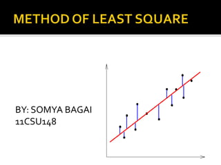
 A CURVE OF “BEST FIT “WHICH CAN PASSTHROUGH
MOST OFTHE POINTS OF GIVEN DATA (OR NEAREST)
IS DRAWN .PROCESS OF FINDING SUCH EQUATION
IS CALLED AS CURVE FITTING .
 THE EQ’N OF THE CURVE IS USED TO FIND
UNKNOWN VALUE.

3.  To find a relationship b/w the set of paired
observations x and y(say), we plot their
corresponding values on the graph , taking one
of the variables along the x-axis and other along
the y-axis i.e. (x1,y1) (X2,Y2)…..,(xn,yn).
 The resulting diagram showing a collection of
dots is called a scatter diagram. A smooth curve
that approximate the above set of points is
known as the approximate curve

4.  LET y=f(x) be equation of curve to be fitted to given data
points at the
experimental value of PM is and the corresponding
value of fitting curve is NM i.e .
),)....(2,2(),1,1( ynxnyxyx xix
yi
)1(xf

5. THIS DIFFERENCE
IS CALLED ERROR.
Similarly we say:
To make all errors
positive ,we square
each of them .
eMINMIPPN 11
)(
)2(22
)1(11
xnfynen
xfye
xfye
2^.........2^32^22^1 eneeeS
THE CURVE OF BEST FIT IS THAT FOR WHICH THE SUM OF
SQUARE OF ERRORS IS MINIMUM .THIS IS CALLED THE
PRINCIPLE OF LEAST SQUARES.

6. METHOD OF LEAST
SQUARE
bxayLET be the straight line to
given data inputs. (1)
2^.......2^22^1
2)^1(2^1
)(1
111
eneeS
bxaye
bxaye
ytye
2^ei
n
i
bxiayiS
1
2)^(

7. For S to be minimum
(2)
(3)
On simplification of above 2 equations
(4)
(5)
0)(0)1)((2
1
bxayorbxiayi
a
S
n
i
0)2^(0))((2
1
bxaxyorxibxiayi
b
S
n
i
xbnay
2^xbxaxy
EQUATION (4) &(5) ARE NORMAL EQUATIONS
SOLVINGTHEMWILL GIVE USVALUE OF a,b

8. To fit the parabola: y=a+bx+cx2 :
 Form the normal equations
 ∑y=na+b∑x+c∑x2 , ∑xy=a∑x+b∑x2 +c∑x3 and
∑x2y=a∑x2 + b∑x3 + c∑x4 .
 Solve these as simultaneous equations for a,b,c.
Substitute the values of a,b,c in y=a+bx+cx2 , which
is the required parabola of the best fit.
 In general, the curve y=a+bx+cx2 +……+kxm-1 can
be fitted to a given data by writing m normal
equations.

9. x y
2 144
3 172.8
4 207.4
5 248.8
6 298.5
Q.FIT A RELATION OF THE FORM ab^x
xBnAY
xBAY
bxay
xaby
lnlnln
^
2^xBxAxY

10. x y Y xY X^2
2 144 4.969 9.939 4
3 172.8 5.152 15.45 9
4 207.4 5.3346 21.3385 16
5 248.8 5.5166 27.5832 25
6 298.5 5.698 34.192 36
20 26.6669 108.504 90
26.67=5A +B20, 108.504=20A+90B
A=4.6044 & B=0.1824
Y=4.605 + x(0.182)
ln y =4.605 +x(0.182)
y= e^(4.605).e^(0.182)

11.  The most important application is in data fitting.
The best fit in the least-squares sense minimizes
the sum of squared residuals, a residual being the
difference between an observed value and the
fitted value provided by a model.
 The graphical method has its drawbacks of being
unable to give a unique curve of fit .It fails to give
us values of unknown constants .principle of least
square provides us with a elegant procedure to do
so.

12. When the problem has substantial uncertainties in
the independent variable (the 'x' variable), then
simple regression and least squares methods have
problems; in such cases, the methodology required for
fitting errors-in-variables models may be considered
instead of that for least squares.