02.bayesian learning

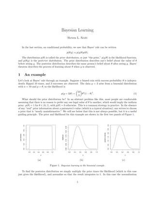
1. Bayesian Learning
Steven L. Scott
In the last section, on conditional probability, we saw that Bayes’ rule can be written
p(θ|y) ∝ p(y|θ)p(θ).
The distribution p(θ) is called the prior distribution, or just “the prior,” p(y|θ) is the likelihood function,
and p(θ|y) is the posterior distribution. The prior distribution describes one’s belief about the value of θ
before seeing y. The posterior distribution describes the same person’s belief about θ after seeing y. Bayes’
theorem describes the process of learning about θ when y is observed.
1 An example
Let’s look at Bayes’ rule through an example. Suppose a biased coin with success probability θ is indepen-
dently flipped 10 times, and 3 successes are observed. The data y = 3 arise from a binomial distribution
with n = 10 and p = θ, so the likelihood is
p(y = 3|θ) =
10
3
θ3
(1 − θ)7
. (1)
What should the prior distribution be? In an abstract problem like this, most people are comfortable
assuming that there is no reason to prefer any one legal value of θ to another, which would imply the uniform
prior: p(θ) = 1 for θ ∈ (0, 1), with p(θ) = 0 otherwise. This is a common strategy in practice. In the absence
of any “real” prior information about a parameter’s value (which is a typical situation), one strives to choose
a prior that is “nearly noninformative.” We will see below that this is not always possible, but it is a useful
guiding principle. The prior and likelihood for this example are shown in the first two panels of Figure 1.
0.0 0.2 0.4 0.6 0.8 1.0
0.00.20.40.60.81.0
θ
priordensity
0.0 0.2 0.4 0.6 0.8 1.0
0.000.050.100.150.200.25
θ
likelihood
0.0 0.2 0.4 0.6 0.8 1.0
0.00.51.01.52.02.53.0
θ
posteriordensity
(a) (b) (c)
Figure 1: Bayesian learning in the binomial example.
To find the posterior distribution we simply multiply the prior times the likelihood (which in this case
just gives the likelihood), and normalize so that the result integrates to 1. In this case the normalization
1

2. constant is proportional to a mathematical special function known as the “beta function”, and the resulting
distribution is a known distribution called the “beta distribution.” The density of the beta distribution with
parameters a and b is
p(θ) =
Γ(a + b)
Γ(a)Γ(b)
θa−1
(1 − θ)b−1
. (2)
If θ is a random variable with the density function in equation (2) then we say θ ∼ Be(a, b). If we ignore
factors other than θ and 1−θ we see that in our example a−1 = 3 and b−1 = 7, so our posterior distribution
must be Be(4, 8). This distribution is plotted in Figure 1(c). Because it is simply a renormalization of the
function in Figure 1(b), the two panels differ only in the axis labels.
2 Conjugate priors
The uniform prior used in the previous section would be inappropriate if we actually had prior information
that θ was small. For example, if y counted conversions on a website, we might have historical information
about the distribution of conversion rates on similar sites. If we can describe our prior belief in the form of
a Be(a, b) distribution (i.e. if we can represent our prior beliefs by choosing specific numerical values of a
and b), then the posterior distribution after observing y successes out of n binomial trials is
p(θ|y) ∝
n
y
θy
(1 − θ)n−y
likelihood
Γ(a + b)
Γ(a)Γ(b)
θa−1
(1 − θ)b−1
prior
∝ θy+a−1
(1 − θ)n−y+b−1
.
(3)
We move from the first line of equation (3) to the second by combining the exponents of θ and 1 − θ, and
ignoring factors that don’t depend on θ. We recognize the outcome as proportional to the Be(y+a, n−y+b)
distribution. Thus “Bayesian learning” in this example amounts to adding y to a and n − y to b. That’s a
helpful way of understanding the prior parameters: a and b represent “prior successes” and “prior failures.”
When Bayes’ rule combines a likelihood and a prior in such a way that the posterior is from the same
model family as the prior, the prior is said to be conjugate to the likelihood. Most models don’t have
conjugate priors, but many models in the exponential family do. A distribution is in the exponential family
if its log density is a linear function of some function of the data. That is, if its density can be written
p(y|θ) = a(θ)b(y)ec(θ) d(y)
. (4)
Many of the famous “named” distributions are in the exponential family, including binomial, Poisson, ex-
ponential, and Gaussian. The student t distribution is an example of a “famous” distribution that is not in
the exponential family.
If a model is in the exponential family then it has sufficient statistics: i d(yi). You can find the
conjugate prior for an exponential family model by imagining equation (4) as a function of θ rather than y,
and renormalizing (assuming the integral with respect to θ is finite). This formulation makes it clear that
the parameters of the prior can be interpreted as sufficient statistics for the model, like how a and b can be
thought of as prior successes and failures in the binomial example.
A second example is the variance of a Gaussian model with known mean. Error terms in many models are
often assumed to be zero-mean Gaussian random variables, so this problem comes up frequently. Suppose
yi ∼ N 0, σ2
, independently, and let y = y1, . . . , yn. The likelihood function is
p(y|σ2
) = (2π)−n/2 1
σ2
n/2
exp −
1
2σ2
i
y2
i . (5)
2

3. Distribution Conjugate Prior
binomial beta
Poisson / exponential gamma
normal mean (known variance) Normal
normal precision (known mean) gamma
Table 1: Some models with conjugate priors
The expression containing 1/σ2
in equation (5) looks like the kernel of the gamma distribution. We write
θ ∼ Ga(a, b) if
p(θ|a, b) =
ba
Γ(a)
θa−1
exp(−bθ). (6)
If one assumes the prior 1/σ2
∼ Ga df
2 , ss
2 then Bayes’ rule gives
p(1/σ2
|y) ∝
1
σ2
n/2
exp −
1
2σ2
i
y2
i
likelihood
1
σ2
df
2 −1
exp −
ss
2
1
σ2
prior
∝
1
σ2
n+df
2 −1
exp −
1
σ2
ss + i y2
i
2
∝ Ga
n + df
2
,
ss + i y2
i
2
.
(7)
Notice how the parameters of the prior df and ss interact with the sufficient statistics of the model. One
can interpret df as a “prior sample size” and ss as a “prior sum of squares.”
It is important to stress that not all models have conjugate priors, and even when they do conjugate
priors may not appropriately express certain types of prior knowledge. Yet when they exist, thinking about
prior distributions through the lens of conjugate priors can help you understand the information content of
the assumed prior.
3 Posteriors compromise between prior and likelihood
Conjugate priors allow us to mathematically study the relationship between prior and likelihood. In the
binomial example with a beta prior, the Be(a, b) distribution has mean π = a/(a + b) and variance π(1 −
π)/(ν + 1), where ν = a + b. It is clear from equation (3) that a acts like a prior number of successes and b
a prior number of failures. The mean of the posterior distribution Be(a + y, b + n − y) is thus
˜π =
a + y
ν + n
= ν
a/ν
ν + n
+ n
y/n
ν + n
. (8)
Equation (8) shows the posterior mean θ is a weighted average of the prior mean a/ν and the mean of the
data y/n. The weights in the average are proportional to ν and n, which are the total information content
in the prior and the data, respectively.
The posterior variance is
˜π(1 − ˜π)
n + ν + 1
. (9)
The total amount of information in the posterior distribution is often measured by its precision, which is the
inverse (reciprocal) of its variance. The precision of Be(a + y, b + n − y) is
n
˜π(1 − ˜π)
+
ν + 1
˜π(1 − ˜π)
,
3

4. which is the sum of the precision from the prior and from the data.
The results shown above are not specific to the binomial distribution. In the general setting, the posterior
mean is a precision weighted average of the mean from the data and the mean from the prior, while the
inverse of the posterior variance is the sum of the prior precision and data precision. This fact helps us get
a sense of the relative importance of the prior vs the data in forming the posteriror distribution.
4 How much should you worry about the prior?
People new to Bayesian reasoning are often concerned about “assuming the answer,” in the sense that their
choice of a prior distribution will unduly influence the posterior distribution. There is good news and bad
on this front.
4.1 Likelihood dominates prior
First the good news. In regular models with moderate to large amounts of data, the data asymptotically
overwhelm the prior. Consider Figure 2, which compares a few different Beta prior distributions with the
same data, to see impact on the posterior. In panel (a) the data contain only 10 observations, so varying the
a and b parameters in the prior distribution by one or two units each represents an appreciable change in
the total available information. Panel2(b) shows the same analysis when there are 100 observations in the
data, so moving a prior parameter by one or two units doesn’t have a particularly big impact.
0.0 0.2 0.4 0.6 0.8 1.0
0.00.51.01.52.02.53.0
θ
density
Be(1, 1)
Be(.5, .5)
Be(2, .5)
Be(.5, 2)
0.0 0.2 0.4 0.6 0.8 1.0
02468
θ
density
Be(1, 1)
Be(.5, .5)
Be(2, .5)
Be(.5, 2)
(a) (b)
Figure 2: How the posterior distributions varies with the choice of prior. (a) 3 successes from 10 trials, (b) 30
successes from 100 trials.
Whatever prior you choose contains a fixed amount of information. If you imagine applying that prior
to larger and larger data sets, its influence will eventually vanish.
4

5. 4.2 Sometimes priors do strange things
Now for the bad news. Even though many models are insensitive to a poorly chosen prior, not all of them
are. If your model is based on means, standard deviations, and regression coefficients, then there is a good
chance that any “weak” prior that you choose will have minimal impact. If the model has lots of latent
variables and other weakly identified unknowns, then the prior is probably more influential. Because priors
can sometimes carry more influence than intended, researchers have spent a considerable amount of time
thinking about how to best represent “prior ignorance” using a default prior. Kass and Wasserman 1996
ably summarize these efforts.
One issue that can come up is that the amount of information in a prior distributions can depend on
the scale in which one views a parameter. For example suppose you place a uniform prior on θ, but then
the analysis calls for the distribution of z = log(θ/(1 − θ)). The Jacobian of this transformation implies
f(z) = θ(1−θ), which is plotted (as a function of z) in Figure 3. The uniform prior on θ is clearly informative
for logit(θ).
−10 −5 0 5 10
0.000.050.100.150.200.25
z
density
Figure 3: The solid line shows the density of a uniform random variable on the logit scale, derived mathematically.
The histogram is the logit transform of 10,000 uniform random deviates.
4.3 Should you worry about priors?
Sometimes you need to, and sometimes you don’t. Until you get enough experience to trust your intuition
about whether a prior is worth worrying about, it is prudent to try an analysis under a few different choices
of prior. You can vary the prior parameters among a few reasonable values, or you can experiment to see
just how extreme the prior would need to be to derail the analysis.
In their paper, Kass and Wasserman made the point that problems where weak priors can make a big
difference tend to be “hard” problems where there is not much information in the data, in which case a
non-Bayesian analysis wouldn’t be particularly compelling (or in some cases, wouldn’t be possible). If you
find that modest variations in the prior lead to different conclusions, then you’re in a hard problem. In that
case a practical strategy is to think about the scale on which you want to analyze your model, and choose
a prior that represents reasonable assumptions on that scale. State your assumptions up front, and present
5

6. the results with a 2-3 other prior choices to show their impact. Then proceed with your chosen prior for the
rest of the analysis.
6