SlideShare une entreprise Scribd logo
1  sur  64
In any element (or in any bounded system), the equation of mass
balance is simply
(Rate of mass flow in) – (Rate of mass flow out) = (Rate of mass
accumulation)
MASS BALANCE IN A FLOWING FLUID; CONTINUITY
𝜌𝑢 𝑥 𝜌𝑢 𝑥+∆𝑥
𝑥, 𝑦, 𝑧
𝑥 + ∆𝑥, 𝑦 + ∆𝑦, 𝑧 + ∆𝑧
∆𝑥
∆𝑧
∆𝑦
𝑥
𝑧
𝑦
𝜌𝑤 𝑧
𝜌𝑤 𝑧+∆𝑧
𝜌𝑣 𝑦
𝜌𝑣 𝑦+∆𝑦
Flux is defined as the rate of flow of any quantity per unit area.
For a fluid of density 𝜌 in 𝑥 direction
the mass flux in 𝑥 direction at the face 𝑥 is 𝜌𝑢 𝑥 ;
the mass flux in 𝑥 direction at the face 𝑥+ ∆𝑥 is 𝜌𝑢 𝑥+∆𝑥;
The rate of mass flow entering the element in 𝑥 direction 𝜌𝑢 𝑥 ∆𝑦∆𝑧 ;
The rate of mass flow leaving the element in 𝑥 direction 𝜌𝑢 𝑥+∆𝑥∆𝑦∆𝑧;
The rate of accumulation in the volume element is ∆𝑥∆𝑦∆𝑧
𝜕𝜌
𝜕𝑡
For a fluid of density 𝜌 in 𝑦 direction
the mass flux in 𝑦 direction at the face 𝑦 is 𝜌𝑣 𝑦 ;
the mass flux in 𝑦 direction at the face 𝑦+ ∆𝑦 is 𝜌𝑣 𝑦+∆𝑦;
The rate of mass flow entering the element in 𝑦 direction 𝜌𝑣 𝑦 ∆𝑥∆𝑧 ;
The rate of mass flow leaving the element in 𝑦 direction 𝜌𝑣 𝑦+∆𝑦∆𝑥∆𝑧;
Similar terms can be obtained for a fluid in 𝑧 direction (𝑤 is velocity)
𝜌𝑢 𝑥 − 𝜌𝑢 𝑥+∆𝑥 ∆𝑦∆𝑧 + 𝜌𝑣 𝑦 − 𝜌𝑣 𝑦+∆𝑦 ∆𝑥∆𝑧
+ 𝜌𝑤 𝑧 − 𝜌𝑤 𝑧+∆𝑧 ∆𝑥∆𝑦 = ∆𝑥∆𝑦∆𝑧
𝜕𝜌
𝜕𝑡
𝜌𝑢 𝑥 − 𝜌𝑢 𝑥+∆𝑥
∆𝑥
+
𝜌𝑣 𝑦 − 𝜌𝑣 𝑦+∆𝑦
∆𝑦
+
𝜌𝑤 𝑧 − 𝜌𝑤 𝑧+∆𝑧
∆𝑧
=
𝜕𝜌
𝜕𝑡
𝜕𝜌
𝜕𝑡
= −
𝜕 𝜌𝑢
𝜕𝑥
+
𝜕 𝜌𝑣
𝜕𝑦
+
𝜕 𝜌𝑤
𝜕𝑧
= − ∇ ∙ 𝜌𝑉
The above equation is known as the equation of continuity. The quantity
∇ ∙ 𝜌𝑉 on the right hand side denotes the divergence of the mass velocity
vector 𝜌𝑉.
Taking the limit as ∆𝑥 , ∆𝑦 , and ∆𝑧 approach zero gives the differential
equation of conservation of mass in a fluid.
Dividing through ∆𝑥 ∆𝑦 ∆𝑧 gives.
𝜕𝜌
𝜕𝑡
= − 𝜌
𝜕𝑢
𝜕𝑥
+ 𝑢
𝜕𝜌
𝜕𝑥
− 𝜌
𝜕𝑣
𝜕𝑦
+ 𝑣
𝜕𝜌
𝜕𝑦
− 𝜌
𝜕𝑤
𝜕𝑧
+ 𝑤
𝜕𝜌
𝜕𝑧
𝜕𝜌
𝜕𝑡
+ 𝑢
𝜕𝜌
𝜕𝑥
+ 𝑣
𝜕𝜌
𝜕𝑦
+ 𝑤
𝜕𝜌
𝜕𝑧
= −𝜌
𝜕𝑢
𝜕𝑥
+
𝜕𝑣
𝜕𝑦
+
𝜕𝑤
𝜕𝑧
𝐷𝜌
𝐷𝑡
= −𝜌
𝜕𝑢
𝜕𝑥
+
𝜕𝑣
𝜕𝑦
+
𝜕𝑤
𝜕𝑧
= −𝜌 ∇ ∙ 𝑉
∇ ∙ 𝑉 =
𝜕𝑢
𝜕𝑥
+
𝜕𝑣
𝜕𝑦
+
𝜕𝑤
𝜕𝑧
= 0
Continuity equation for a fluid with constant density. Often in engineering
the fluid is almost incompressible and density may be considered constant
Where Dρ/Dt is the substantial derivative or the derivative following the
motion. At steady state
𝜕𝜌
𝜕𝑡
= 0.
Carrying out the partial differentiation gives
A stream line is an imaginary curve in a mass of flowing fluid
so drawn that at every point on the curve, the net velocity vector
is tangent to the stream line as shown in figure
No net flow takes place across such a line.
In turbulent flow, eddies do cross and recross a streamline, however,
the net flow from such eddies is zero.
One dimensional flow
A stream tube, or stream filament, is a tube of any convenient cross-
section and shape that is entirely bounded by stream lines. A stream
tube can be visualized as an imaginary pipe in the mass of flowing
fluid through the walls of which no net flow is occurring. If the tube
has a differential cross-sectional area dS, the velocity through the tube
can also be denoted by a single term u.
The mass flow through the differential are is
𝑑𝑚 = 𝜌𝑢 𝑑𝑆
If the fluid is heated or cooled, the fluid density varies, but
usually the variation is small and can be neglected.
𝑚 = 𝜌
𝑆
𝑢 𝑑𝑆
𝑉 ≡
𝑚
𝜌𝑆
=
1
𝑆 𝑆
𝑢 𝑑𝑆
𝑉 =
𝑞
𝑆
The velocity 𝑉 also equals the volumetric flow rate divided by the
cross-sectional area of the conduit
It is also flux of volume or volume flux
The average velocity 𝑉 of the entire stream flowing through a
cross-sectional area S is defined by
The flow rate through entire crosssection is
𝜌𝑏 𝑉𝑏
𝑆𝑏
𝑚 = 𝜌𝑎𝑆𝑎𝑉
𝑎= 𝜌𝑏𝑆𝑏𝑉𝑏 = 𝜌𝑆𝑉
𝑚 =
𝜋
4
𝐷𝑎
2𝜌𝑎𝑉
𝑎=
𝜋
4
𝐷𝑏
2
𝜌𝑏𝑉𝑏
𝜌𝑎𝑉
𝑎 𝐷𝑎
2 = 𝜌𝑏𝑉𝑏𝐷𝑏
2
𝜌𝑎𝑉𝑎
𝜌𝑏𝑉𝑏
=
𝐷𝑏
𝐷𝑎
2
𝑉𝑎
𝑉𝑏
=
𝐷𝑏
𝐷𝑎
2
Shell balance for mass flow
Consider the system as shown in the figure below
𝑆𝑎
𝑉
𝑎 𝜌𝑎
Flow through circular cross section
At steady state mass flow in is equal to mass flow out and the continuity
equation becomes
If density remains constant than
Shell balance is
𝐺 ≡
𝑚
𝑆
= 𝑉𝜌
Mass velocity
In practice the mass velocity is expressed as kilograms per square
meter per second, pounds per square foot per second.
The advantage of using G is that it is independent of temperature and
pressure when flow is steady (constant 𝑚) and the cross section is
unchanged (Constant S).
This fact is useful when compressible fluids are considered, for both
𝑉 and 𝜌 vary with temperature and pressure.
The mass velocity G can also be described as mass current density or
mass flux.
A momentum balance may be made on a volume element in much the
same way as a mass balance, but since velocity is a vector, the
derivation is considerably complicated. The basic concept of the
momentum balance is as follows
DIFFERENTIAL MOMENTUM BALANCE;
EQUATIONS OF MOTION
Rate of
momentum
accumulation
=
Rate of
momentum
leaving
sum of forces
acting on the
system
+
-
The fluid is flowing through all six faces of the volume element in any
arbitrary direction. Since velocity is a vector, Equation 1 has
components in each of coordinate direction x,y, and z. First we
consider only the x component of each term in Equation 1, the y and z
components may be treated analogously.
Rate of
momentum
entering
𝜌𝑢𝑢 𝑥 𝜌𝑢𝑢 𝑥+∆𝑥
𝑥, 𝑦, 𝑧
𝑥 + ∆𝑥, 𝑦 + ∆𝑦, 𝑧 + ∆𝑧
∆𝑥
∆𝑧
∆𝑦
𝑥
𝑧
𝑦
𝜌𝑤𝑢 𝑧
𝜌𝑤𝑢 𝑧+∆𝑧
𝜌𝑣𝑢 𝑦
𝜌𝑣𝑢 𝑦+∆𝑦
For a fluid of density 𝜌 in 𝑥 direction
The rate at which the x component of momentum enters the face at x by
convection is 𝜌𝑢𝑢 𝑥 ∆𝑦∆𝑧 ;
The rate at which it leaves at 𝑥+ ∆𝑥 is 𝜌𝑢𝑢 𝑥+∆𝑥∆𝑦∆𝑧;
The rate at which the x component of momentum enters the face at x by
convection is 𝜌𝑤𝑢 𝑧 ∆𝑥∆𝑦 ;
The rate at which it leaves at 𝑧+ ∆𝑧 is 𝜌𝑤𝑢 𝑧+∆𝑧∆𝑥∆𝑦;
The rate at which the x component of momentum enters the face at y by
convection is 𝜌𝑣𝑢 𝑦 ∆𝑥∆𝑧 ;
The rate at which it leaves at 𝑦+ ∆𝑦 is 𝜌𝑣𝑢 𝑦+∆𝑦∆𝑥∆𝑧;
Department of Chemical Engineering, AU College of Engineering (A)
The rate of accumulation of momentum in the volume element is
∆𝑥∆𝑦∆𝑧
𝜕
𝜕𝑡
𝜌𝑢
𝜌𝑢𝑢 𝑥 − 𝜌𝑢𝑢 𝑥+∆𝑥 ∆𝑦∆𝑧 + 𝜌𝑣𝑢 𝑦 − 𝜌𝑣𝑢 𝑦+∆𝑦 ∆𝑥∆𝑧
+ 𝜌𝑤𝑢 𝑧 − 𝜌𝑤𝑢 𝑧+∆𝑧 ∆𝑥∆𝑦
The net convective flow into the volume element is
𝜏𝑥𝑥 𝑥 𝜏𝑥𝑥 𝑥+∆𝑥
∆𝑥
∆𝑧
∆𝑦
𝑥
𝑧
𝑦
𝜏𝑧𝑥 𝑧
𝜏𝑧𝑥 𝑧+∆𝑧
𝜏𝑦𝑥 𝑦
𝜏𝑦𝑥 𝑦+∆𝑦
The rate at which the x component of momentum enters the face at x by
molecular transport/Viscous forces is 𝜏𝑥𝑥 𝑥∆𝑦∆𝑧
and the rate at which it leaves at 𝑥 + ∆𝑥 is 𝜏𝑥𝑥 𝑥+∆𝑥∆𝑦∆𝑧 ;
Considering x component in three directions x, y, and z
The rate at which the x component of momentum enters the face at y by
molecular transport/Viscous forces is 𝜏𝑦𝑥 𝑦
∆𝑥∆𝑧
and the rate at which it leaves at 𝑦 + ∆𝑦 is 𝜏𝑦𝑥 𝑦+∆𝑦
∆𝑥∆𝑧 ;
The rate at which the x component of momentum enters the face at z by
molecular transport/Viscous forces is 𝜏𝑧𝑥 𝑧∆𝑥∆𝑦
and the rate at which it leaves at 𝑧 + ∆𝑧 is 𝜏𝑧𝑥 𝑧+∆𝑧∆𝑥∆𝑦 ;
𝜏𝑥𝑥 𝑥 − 𝜏𝑥𝑥 𝑥+∆𝑥 ∆𝑦∆𝑧 + 𝜏𝑦𝑥 𝑦
− 𝜏𝑦𝑥 𝑦+∆𝑦
∆𝑥∆𝑧
+ 𝜏𝑧𝑥 𝑧 − 𝜏𝑧𝑥 𝑧+∆𝑧 ∆𝑥∆𝑦
Summing up these six contributions gives the net flow of x
momentum into the volume element by viscous action:
In most cases the important forces acting on the system arise from the
fluid pressure 𝑝 and the gravitational force per unit mass g. the
resultant of the forces in x direction is
𝑝 𝑥 − 𝑝 𝑥+∆𝑥 ∆𝑦∆𝑧 + ρ𝑔𝑥∆𝑥∆𝑦∆𝑧
∆𝑥∆𝑦∆𝑧
𝜕
𝜕𝑡
𝜌𝑢 = 𝜌𝑢𝑢 𝑥 − 𝜌𝑢𝑢 𝑥+∆𝑥 ∆𝑦∆𝑧
+ 𝜌𝑣𝑢 𝑦 − 𝜌𝑣𝑢 𝑦+∆𝑦 ∆𝑥∆𝑧
+ 𝜌𝑤𝑢 𝑧 − 𝜌𝑤𝑢 𝑧+∆𝑧 ∆𝑥∆𝑦
+ 𝜏𝑥𝑥 𝑥 − 𝜏𝑥𝑥 𝑥+∆𝑥 ∆𝑦∆𝑧
+ 𝜏𝑦𝑥 𝑦
− 𝜏𝑦𝑥 𝑦+∆𝑦
∆𝑥∆𝑧
+ 𝜏𝑧𝑥 𝑧 − 𝜏𝑧𝑥 𝑧+∆𝑧 ∆𝑥∆𝑦
+ 𝑝 𝑥 − 𝑝 𝑥+∆𝑥 ∆𝑦∆𝑧 + ρ𝑔𝑥∆𝑥∆𝑦∆𝑧
Dividing through ∆𝑥 ∆𝑦 ∆𝑧 Taking the limit as ∆𝑥 , ∆𝑦 , and ∆𝑧
approach zero gives the differential equation of momentum.
𝜕
𝜕𝑡
𝜌𝑢 = −
𝜕
𝜕𝑥
𝜌𝑢𝑢 +
𝜕
𝜕𝑦
𝜌𝑣𝑢 +
𝜕
𝜕𝑧
𝜌𝑤𝑢
−
𝜕
𝜕𝑥
𝜏𝑥𝑥 +
𝜕
𝜕𝑦
𝜏𝑦𝑥 +
𝜕
𝜕𝑧
𝜏𝑧𝑥 −
𝜕𝑝
𝜕𝑥
+ 𝜌𝑔𝑥
𝜌
𝜕𝑢
𝜕𝑡
+ 𝑢
𝜕𝜌
𝜕𝑡
= − 𝑢
𝜕
𝜕𝑥
𝜌𝑢 + 𝑢
𝜕
𝜕𝑦
𝜌𝑣 + 𝑢
𝜕
𝜕𝑧
𝜌𝑤
− 𝜌𝑢
𝜕𝑢
𝜕𝑥
+ 𝜌𝑣
𝜕𝑢
𝜕𝑦
+ 𝜌𝑤
𝜕𝑢
𝜕𝑧
−
𝜕
𝜕𝑥
𝜏𝑥𝑥 +
𝜕
𝜕𝑦
𝜏𝑦𝑥 +
𝜕
𝜕𝑧
𝜏𝑧𝑥 −
𝜕𝑝
𝜕𝑥
+ 𝜌𝑔𝑥
𝜌
𝜕𝑢
𝜕𝑡
+ 𝑢
𝜕𝜌
𝜕𝑡
= −𝑢 −
𝜕𝜌
𝜕𝑡
−𝜌 𝑢
𝜕𝑢
𝜕𝑥
+ 𝑣
𝜕𝑢
𝜕𝑦
+ 𝑤
𝜕𝑢
𝜕𝑧
−
𝜕
𝜕𝑥
𝜏𝑥𝑥 +
𝜕
𝜕𝑦
𝜏𝑦𝑥 +
𝜕
𝜕𝑧
𝜏𝑧𝑥 −
𝜕𝑝
𝜕𝑥
+ 𝜌𝑔𝑥
𝜌
𝜕𝑢
𝜕𝑡
+ 𝑢
𝜕𝑢
𝜕𝑥
+ 𝑣
𝜕𝑢
𝜕𝑦
+ 𝑤
𝜕𝑢
𝜕𝑧
=
−
𝜕
𝜕𝑥
𝜏𝑥𝑥 +
𝜕
𝜕𝑦
𝜏𝑦𝑥 +
𝜕
𝜕𝑧
𝜏𝑧𝑥 −
𝜕𝑝
𝜕𝑥
+ 𝜌𝑔𝑥
𝜌
𝐷𝑢
𝐷𝑡
= −
𝜕
𝜕𝑥
𝜏𝑥𝑥 +
𝜕
𝜕𝑦
𝜏𝑦𝑥 +
𝜕
𝜕𝑧
𝜏𝑧𝑥 −
𝜕𝑝
𝜕𝑥
+ 𝜌𝑔𝑥
𝜌
𝐷𝑣
𝐷𝑡
= −
𝜕
𝜕𝑥
𝜏𝑥𝑦 +
𝜕
𝜕𝑦
𝜏𝑦𝑦 +
𝜕
𝜕𝑧
𝜏𝑧𝑦 −
𝜕𝑝
𝜕𝑦
+ 𝜌𝑔𝑦
𝜌
𝐷𝑤
𝐷𝑡
= −
𝜕
𝜕𝑥
𝜏𝑥𝑧 +
𝜕
𝜕𝑦
𝜏𝑦𝑧 +
𝜕
𝜕𝑧
𝜏𝑧𝑧 −
𝜕𝑝
𝜕𝑧
+ 𝜌𝑔𝑧
𝜌
𝐷𝑉
𝐷𝑡
= −∇𝑝 − ∇. 𝜏 + 𝜌𝑔
𝜏𝑥𝑥 = −2𝜇
𝜕𝑢
𝜕𝑥
+
2
3
𝜇 − 𝑘 ∇. 𝑉 𝜏𝑥𝑦 = 𝜏𝑦𝑥 = 𝜇
𝜕𝑢
𝜕𝑦
+
𝜕𝑣
𝜕𝑥
∇. 𝑉 =
𝜕𝑢
𝜕𝑥
+
𝜕𝑣
𝜕𝑦
+
𝜕𝑤
𝜕𝑧
𝜌
𝐷𝑢
𝐷𝑡
= −
𝜕𝑝
𝜕𝑥
+
𝜕
𝜕𝑥
2𝜇
𝜕𝑢
𝜕𝑥
−
2
3
𝜇 − 𝑘 ∇. 𝑉
+
𝜕
𝜕𝑦
𝜇
𝜕𝑢
𝜕𝑦
+
𝜕𝑣
𝜕𝑥
+
𝜕
𝜕𝑧
𝜇
𝜕𝑤
𝜕𝑥
+
𝜕𝑢
𝜕𝑧
+ 𝜌𝑔𝑥
𝜏𝑧𝑥 = 𝜏𝑥𝑧 = 𝜇
𝜕𝑤
𝜕𝑥
+
𝜕𝑢
𝜕𝑧
For Newtonian fluids the x direction components of stress tensor are
Where k is the bulk viscosity. The general equations for a Newtonian
fluid with varying density and viscosity are exemplified by the
following equation for the x direction.
𝜏𝑥𝑦 = 𝜏𝑦𝑥 = 𝜇
𝜕𝑢
𝜕𝑦
+
𝜕𝑣
𝜕𝑥
∇. 𝑉 =
𝜕𝑢
𝜕𝑥
+
𝜕𝑣
𝜕𝑦
+
𝜕𝑤
𝜕𝑧
𝜌
𝐷𝑣
𝐷𝑡
= −
𝜕𝑝
𝜕𝑦
+
𝜕
𝜕𝑥
𝜇
𝜕𝑢
𝜕𝑦
+
𝜕𝑣
𝜕𝑥
+
𝜕
𝜕𝑦
2𝜇
𝜕𝑣
𝜕𝑥
−
2
3
𝜇 − 𝑘 ∇. 𝑉
+
𝜕
𝜕𝑧
𝜇
𝜕𝑤
𝜕𝑦
+
𝜕𝑣
𝜕𝑧
+ 𝜌𝑔𝑦
𝜏𝑦𝑧 = 𝜏𝑧𝑦 = 𝜇
𝜕𝑣
𝜕𝑧
+
𝜕𝑤
𝜕𝑦
𝜏𝑦𝑦 = −2𝜇
𝜕𝑣
𝜕𝑦
+
2
3
𝜇 − 𝑘 ∇. 𝑉
∇. 𝑉 =
𝜕𝑢
𝜕𝑥
+
𝜕𝑣
𝜕𝑦
+
𝜕𝑤
𝜕𝑧
𝜏𝑦𝑧 = 𝜏𝑧𝑦 = 𝜇
𝜕𝑣
𝜕𝑧
+
𝜕𝑤
𝜕𝑦
𝜏𝑧𝑥 = 𝜏𝑥𝑧 = 𝜇
𝜕𝑤
𝜕𝑥
+
𝜕𝑢
𝜕𝑧
𝜏𝑧𝑧 = −2𝜇
𝜕𝑤
𝜕𝑧
+
2
3
𝜇 − 𝑘 ∇. 𝑉
𝜌
𝐷𝑤
𝐷𝑡
= −
𝜕𝑝
𝜕𝑧
+
𝜕
𝜕𝑥
𝜇
𝜕𝑤
𝜕𝑥
+
𝜕𝑢
𝜕𝑧
+
𝜕
𝜕𝑦
𝜇
𝜕𝑤
𝜕𝑦
+
𝜕𝑣
𝜕𝑧
+
𝜕
𝜕𝑧
2𝜇
𝜕𝑣
𝜕𝑧
−
2
3
𝜇 − 𝑘 ∇. 𝑉 + 𝜌𝑔𝑧
Navier Stokes equations. The previous equations are used in their
complete form only in setting up highly complicated flow problems.
In most situations restricted forms suffice. For a fluid of constant
density and viscosity, the equations of motion, known as navier-stokes
equations, are
𝜌
𝜕𝑢
𝜕𝑡
+ 𝑢
𝜕𝑢
𝜕𝑥
+ 𝑣
𝜕𝑢
𝜕𝑦
+ 𝑤
𝜕𝑢
𝜕𝑧
= 𝜇
𝜕2𝑢
𝜕𝑥
+
𝜕2𝑢
𝜕𝑦
+
𝜕2𝑢
𝜕𝑧
−
𝜕𝑝
𝜕𝑥
+ 𝜌𝑔𝑥
𝜌
𝜕𝑣
𝜕𝑡
+ 𝑢
𝜕𝑣
𝜕𝑥
+ 𝑣
𝜕𝑣
𝜕𝑦
+ 𝑤
𝜕𝑣
𝜕𝑧
= 𝜇
𝜕2𝑣
𝜕𝑥
+
𝜕2𝑣
𝜕𝑦
+
𝜕2𝑣
𝜕𝑧
−
𝜕𝑝
𝜕𝑦
+ 𝜌𝑔𝑦
𝜌
𝜕𝑤
𝜕𝑡
+ 𝑢
𝜕𝑤
𝜕𝑥
+ 𝑣
𝜕𝑤
𝜕𝑦
+ 𝑤
𝜕𝑤
𝜕𝑧
= 𝜇
𝜕2𝑤
𝜕𝑥
+
𝜕2𝑤
𝜕𝑦
+
𝜕2𝑤
𝜕𝑧
−
𝜕𝑝
𝜕𝑧
+ 𝜌𝑔𝑧
In vector form these equations become
𝜌
𝐷𝑉
𝐷𝑡
= −∇𝑝 − 𝜇∇2
𝑽 + 𝜌𝒈
Euler’s equation. For constant density and zero viscosity, as in
potential flow, the equation of motion known as Euler equation , is
𝜌
𝐷𝑉
𝐷𝑡
= −∇𝑝 + 𝜌𝒈
𝜌
𝜕𝑢
𝜕𝑡
+ 𝑢
𝜕𝑢
𝜕𝑥
+ 𝑣
𝜕𝑢
𝜕𝑦
+ 𝑤
𝜕𝑢
𝜕𝑧
= −
𝜕𝑝
𝜕𝑥
+ 𝜌𝑔𝑥
𝐹 = 𝑀𝑏 − 𝑀𝑎
MACROSCOPIC MOMENTUM BALANCES
An overall momentum balance can be written for the control volume
shown in figure, assuming that the flow is steady and unidirectional in
the x direction. The sum of the forces acting on the fluid in the x
direction equals the increase in the momentum flow rate of the fluid
The momentum flow rate 𝑀 of a fluid stream having a mass flow rate
𝑚 and moving at a velocity u is 𝑚𝑢 . If u varies from point to point in
the cross-section of the stream, however, the total momentum does not
equal the product of mass flow rate and the average velocity, or 𝑚𝑉. In
general some what greater than this.
𝑑𝑀
𝑑𝑆
= 𝜌𝑢 𝑢 = 𝜌𝑢2
𝑀
𝑆
=
𝜌 𝑆
𝑢2 𝑑𝑆
𝑆
𝛽 ≡
𝑀
𝑆
𝜌𝑉2
The necessary correction factor is best found from the convective
momentum flux. This is the product of the linear velocity normal to the
cross section and the mass velocity(Mass Flux). For a differential cross
sectional area dS, the momentum flux is
The momentum flux of the whole stream,
for constant density fluid, is
The momentum correction factor is
defined by
𝛽 =
𝜌 𝑆
𝑢2 𝑑𝑆
𝑆
𝜌𝑉2
=
1
𝑆 𝑆
𝑢
𝑉
2
𝑑𝑆
𝐹 = 𝑚 𝛽𝑏𝑉𝑏 − 𝛽𝑎𝑉
𝑎
𝐹 = 𝑝𝑎𝑆𝑎 − 𝑝𝑏𝑆𝑏 + 𝐹𝑤 − 𝐹
𝑔
𝑚 𝛽𝑏𝑉𝑏 − 𝛽𝑎𝑉
𝑎 = 𝑝𝑎𝑆𝑎 − 𝑝𝑏𝑆𝑏 + 𝐹𝑤 − 𝐹
𝑔
The modified momentum balance with correction factor is
The forces acting on the system are
1. Pressure change in the direction of the flow
2. Shear stress at the boundary between fluid stream and the conduit
3. If the stream is inclined the appropriate component of force of
gravity.
4.2. For a given fluid and a given distance between plates in a system
like that shown in Figure 4.5. velocity 𝑣𝑜 must be large enough to
counteract the effect of gravity; otherwise, some of the fluid will flow
downward. In a particular system, the distance between plates is1 mm,
and the fluid is an oil with a density of 900 kg/m3 and a viscosity of 50
mPa-s. The pressure drop 𝑑𝑝 𝑑𝑦 is negligible compared with the term
𝜌𝑔. (a) What is the minimum upward velocity of the moving plate so
that all the fluid moves upward? (b) if 𝑣𝑜 is set at this minimum value,
what is the fluid velocity midway between the plates? (c) What is the
shear rate in the fluid at a stationary plate, at the moving plate, and
midway between them? Use the equations in Example 4.3
Given Data
Distance between plates = 1mm = 0.001 m
Density of the oil ρ = 900 kg/m3
Viscosity of the oil 𝜇 = 50 mPa.S = 50 x 10-3 Pa-s
(a) For none of the liquid to be flowing down dv/dx must be greater
than or equal to zero at x=0. Also
𝜕𝑝
𝜕𝑦
can be neglected when
compared with 𝜌𝑔.
𝜕𝑣
𝜕𝑥
−
𝑥
𝜇
𝜕𝑝
𝜕𝑦
+ 𝜌𝑔 = 𝐶1 =
𝑣𝑜
𝐵
−
𝐵
2𝜇
𝜕𝑝
𝜕𝑦
+ 𝜌𝑔
𝜕𝑣
𝜕𝑥
= 0 =
𝑣𝑜
𝐵
−
𝐵𝜌𝑔
2𝜇
𝑣𝑜
𝐵
=
𝐵𝜌𝑔
2𝜇
𝑣𝑜 =
𝐵2𝜌𝑔
2𝜇
=
0.00120.001900𝑥9.8065
2𝑥0.05
= 0.08826
𝑚
𝑠
= 88.26 𝑚𝑚/𝑠
(b) The velocity at midway (x = B/2) is evaluated from the formula
𝑣 = 𝑣𝑜
𝑥
𝐵
−
1
2𝜇
𝜕𝑝
𝜕𝑦
+ 𝜌𝑔 𝐵𝑥 − 𝑥2
𝑣 = 𝑣𝑜
𝐵
2𝐵
−
1
2𝜇
𝜌𝑔 𝐵
𝐵
2
−
𝐵
2
2
𝑣 =
𝑣𝑜
2
−
𝜌𝑔
2𝜇
𝐵2
4
𝑣 =
𝑣𝑜
2
−
𝑣𝑜
4
=
𝑣𝑜
4
=
0.08826
4
= 0.02206
𝑚
𝑠
= 22.06 𝑚𝑚/𝑠
4.9. The velocity profile in a fluid stream is approximated using a
three part model, where the velocity is 1.6m/s in 15 percent cross-
sectional area, 3.2m/s in 35 percent of the area, and 4.5m/s in the rest
of the area. (a) How much does the total momentum of the fluid differ
from the product of the mass flow rate and the average velocity? (b)
Can you think of a situation where there is a velocity profile in the
flow stream and the momentum flow is exactly equal to the mass flow
times the average velocity?
Given data
Velocity of fluid for 15% 𝑉= 1.6 m/s
Velocity of fluid for 35% 𝑉= 3.2 m/s
Velocity of fluid for 50% 𝑉= 4.5 m/s
Assume total cross-sectional area be S, Then
Flow rate for 15 % area Q1 =1.6 x 0.15 =0.24S
Flow rate for 35 % area Q2 =3.2 x 0.35 =1.12S
Flow rate for 50 % area Q2 =4.5 x 0.50 =2.25S
Total flow rate Q = 0.24S + 1.12S + 2.25S = 3.61S
Average Velocity 𝑉 = Q/S = 3.61S/S = 3.61 m/s
Momentum developed in 15 % area
𝑚1
𝜌
= 1.62𝑥0.15𝑆 = 0.384𝑆
Momentum developed in 35 % area
𝑚2
𝜌
= 3.22
𝑥0.35𝑆 = 3.584𝑆
Momentum developed in 50 % area
𝑚3
𝜌
= 4.52
𝑥0.50𝑆 = 10.125𝑆
Total momentum developed is
𝑚
𝜌
= 0.384𝑆 + 3.584𝑆 + 10.125𝑆 = 14.093𝑆
Total momentum based on average velocity
𝑚
𝜌
= 3.612 𝑆 = 13.0321𝑆
The ratio of momentum based on average velocity to actual Momentum
13.0321
14.093
= 0.9247
The value of beta = 𝛽 =
14.093
13.0321
= 1.0814
The only situation where momentum is calculated from average velocity
is in the plug flow region where velocity is same.
4.5. Water enters a 100-mm-ID 900 elbow, positioned in a horizontal
plane, at a velocity of 6 m/s and a pressure of 70 kN/m2 gauge.
Neglecting friction, what are the magnitude and the direction of the
force that must be applied to the elbow to keep it in position without
moving?
Assume elbow is in the x-z plane with water entering in
the x direction and leaving in the z direction. Since water
flows horizontally Fg is 0.
𝑚 𝛽𝑏𝑉𝑏,𝑥 − 𝛽𝑎𝑉
𝑎,𝑥 = 𝑝𝑎𝑆𝑎,𝑥 − 𝑝𝑏𝑆𝑏,𝑥 + 𝐹𝑤,𝑥
𝑚 𝛽𝑏𝑉𝑏,𝑧 − 𝛽𝑎𝑉
𝑎,𝑧 = 𝑝𝑎𝑆𝑎,𝑧 − 𝑝𝑏𝑆𝑏,𝑧 + 𝐹𝑤,𝑧
Given data
Diameter of the pipe, D = 100 mm = 0.1 m
Cross sectional area of pipe S =
𝜋
4
0.1 2
= 7.854 𝑥 10−3
m2
Velocity of water 𝑉= 6 m/s
Pressure p = 70 kN/m2 = 70,000 N/m2
Mass flow rate 𝑚 = 1000 x 6 x 7.854 𝑥 10−3 = 47.1239 kg/s
Density of water ρ= 1000 kg/m3
Assume 𝛽𝑎 = 𝛽𝑏 = 1
𝑉
𝑎,𝑥 = 𝑉𝑏,𝑧 = 𝑉 = 6 𝑚/𝑠
𝑉𝑏,𝑥 = 𝑉
𝑎,𝑧 = 0 𝑚/𝑠
𝑆𝑎,𝑥 = 𝑆𝑏,𝑧 = 𝑆 = 7.854 𝑥 10−3 m2
𝑆𝑎,𝑧 = 𝑆𝑏,𝑥 = 0 𝑚2
𝐹𝑤,𝑥 = 𝑚 𝛽𝑏𝑉𝑏,𝑥 − 𝛽𝑎𝑉
𝑎,𝑥 − (𝑝𝑎𝑆𝑎,𝑥 − 𝑝𝑏𝑆𝑏,𝑥)
𝐹𝑤,𝑥 = 47.1239 0 − 6 − (70000𝑥0.007854 − 0)
𝐹𝑤,𝑥 = −832.5234 𝑁
𝐹𝑤,𝑧 = 𝑚 𝛽𝑏𝑉𝑏,𝑧 − 𝛽𝑎𝑉
𝑎,𝑧 − 𝑝𝑎𝑆𝑎,𝑧 − 𝑝𝑏𝑆𝑏,𝑧
𝐹𝑤,𝑧 = 47.1239 6 − 0 − 0 − 70000𝑥0.007854
𝐹𝑤,𝑧 = 832.5234 𝑁
832.5234
-832.5234
The total force of 832.5234√2 = 1177.3659 N will be acting in
the direction shown
Department of Chemical Engineering, AU College of Engineering (A)
Layer flow with free surface
𝑚 𝛽𝑏𝑉𝑏 − 𝛽𝑎𝑉
𝑎 = 𝑝𝑎𝑆𝑎 − 𝑝𝑏𝑆𝑏 + 𝐹𝑤 − 𝐹
𝑔
0
Fg
𝐹
𝑔 cos ∅ − 𝜏𝐴 = 0
𝜏𝐿𝑏 = 𝜌𝑟𝐿𝑏𝑔 cos ∅
𝜏 = 𝜌𝑟𝑔 cos ∅
𝜏 = −𝜇
𝑑𝑢
𝑑𝑟
−𝜇
𝑑𝑢
𝑑𝑟
= 𝜌𝑟𝑔 cos ∅
0
𝑢
𝑑𝑢 = −
𝜌𝑔 cos ∅
𝜇 𝛿
𝑟
𝑟 𝑑𝑟
𝑢 = −
𝜌𝑔 cos ∅
2𝜇
𝑟2 − 𝛿2 =
𝜌𝑔 cos ∅
2𝜇
𝛿2 − 𝑟2
𝑚 =
0
𝛿
𝜌𝑢𝑏 𝑑𝑟
𝑚
𝑏
= 𝜌
0
𝛿
𝜌𝑔 cos ∅
2𝜇
𝛿2 − 𝑟2 𝑑𝑟
𝑚
𝑏
=
𝜌2𝑔 cos ∅
2𝜇 0
𝛿
𝛿2 − 𝑟2 𝑑𝑟
𝑚
𝑏
=
𝜌2𝑔 cos ∅
2𝜇
𝛿3
−
𝛿3
3
𝑚
𝑏
= 𝜌
0
𝛿
𝑢 𝑑𝑟
𝑚
𝑏
=
𝛿3
𝜌2
𝑔 cos ∅
3𝜇
= Г
𝛿3 =
3𝜇Г
𝜌2𝑔 cos ∅
𝛿 =
3𝜇Г
𝜌2𝑔 cos ∅
1
3
4.6. A vertical cylinder reactor 2.5 m in diameter and 4 m high is
cooled by spraying water on the top and allowing the water to flow
down the outside wall. The water flow rate is 0.15 m3/min, and the
average water temperature is 40oC. Estimate the thickness of the layer
of water.
𝛿 =
3𝜇Г
𝜌2𝑔 cos ∅
1
3
=
3𝑥0.000656𝑥2.5
10002𝑥9.80665𝑥1
1
3
= 0.000399 = 0.4𝑚𝑚
Volumetric flow rate = 0.15/60 = 0.0025 m3/s
Density of water = 1000 kg/m3
Viscosity of water = 0.656cP = 0.656x10⁻³ Pa-s
Mass flow rate m = 0.0025 x 1000 = 2.5 kg/s
b = (22/7) 2.5 = 7.857 m
MECHANICAL ENERGY EQUATION
Energy equation for potential flow; Bernoulli equation without
friction
The 𝑥 component of the Euler equation is
𝜌
𝜕𝑢
𝜕𝑡
+ 𝑢
𝜕𝑢
𝜕𝑥
+ 𝑣
𝜕𝑢
𝜕𝑦
+ 𝑤
𝜕𝑢
𝜕𝑧
= −
𝜕𝑝
𝜕𝑥
+ 𝜌𝑔𝑥
Department of Chemical Engineering, AU College of Engineering (A)
The unidirectional flow 𝑣 and 𝑤 are zero. Multiplying the remaining
terms by the velocity u gives
𝜌𝑢
𝜕𝑢
𝜕𝑡
+ 𝑢
𝜕𝑢
𝜕𝑥
= −𝑢
𝜕𝑝
𝜕𝑥
+ 𝜌𝑢𝑔𝑥
𝜌
𝜕 𝑢2 2
𝜕𝑡
+ 𝑢
𝜕 𝑢2 2
𝜕𝑥
= −𝑢
𝜕𝑝
𝜕𝑥
+ 𝜌𝑢𝑔𝑥
This is the mechanical energy equation for unidirectional potential of
fluids of constant density when flow rate varies with time.
Consider now a volume element of a stream tube within a larger
stream of fluid, as shown in figure flowing at steady flow. Assume the
cross section of the tube increases continuously in the direction of
flow and that the axis of tube is straight and inclined at an angle 𝝓 as
shown.
Since flow is steady
𝜕𝑢
𝜕𝑡
is zero. Since the flow is Unidirectional u is a
function only of 𝑥. Since gravity acts in negative x direction
𝑔𝑥 = −𝑔 cos ∅ . And cos ∅ = dZ/dx
𝜌
𝜕𝑢
𝜕𝑡
+ 𝑢
𝜕𝑢
𝜕𝑥
+ 𝑣
𝜕𝑢
𝜕𝑦
+ 𝑤
𝜕𝑢
𝜕𝑧
= −
𝜕𝑝
𝜕𝑥
+ 𝜌𝑔𝑥
0 0 0
𝜌 𝑢
𝜕𝑢
𝜕𝑥
= −
𝜕𝑝
𝜕𝑥
− 𝜌𝑔 cos ∅
𝜌
𝑑 𝑢2 2
𝑑𝑥
+
𝑑𝑝
𝑑𝑥
+ 𝜌𝑔
𝑑𝑍
𝑑𝑥
= 0
𝑑 𝑢2
2
𝑑𝑥
+
1
𝜌
𝑑𝑝
𝑑𝑥
+ 𝑔
𝑑𝑍
𝑑𝑥
= 0
Integrating the equation we have
𝑝
𝜌
+ 𝑔𝑍 +
𝑢2
2
= 𝑐𝑜𝑛𝑠𝑡
Integrating over the system shown in fiquare
𝑝𝑎
𝜌
+ 𝑔𝑍𝑎 +
𝑢𝑎
2
2
=
𝑝𝑏
𝜌
+ 𝑔𝑍𝑏 +
𝑢𝑏
2
2
Each term has a units of energy per unit mass
𝑔𝑍 represents Potential energy per unit mass
𝑢2
2
represents Kinetic energy per unit mass
𝑝
𝜌
represents Mechanical work done by forces external to the stream
If velocity is reduced then either the datum height or pressure should
increase or both should increase.
Station a and b are chosen on the basis of convenience and are usall
taken at locations where the most information about pressures,
velocities, and heights are available.
Bernoulli equation: correction for effects of solid boundaries.
To extend the Bernoulli equation to cover the practical situations
streams that are influenced by solid boundaries, two modifications are
needed.
The first is the correction of the kinetic energy term for variation of
local velocity u with position in the boundary layer,
The Second, of major importance , is the correction of equation for
the existence of fluid friction, which appears whenever boundary
layer forms.
Kinetic energy of stream
The term
𝑢2
2
is the kinetic energy of a unit mass of fluid all of which is
flowing at the same velocity 𝑢. when the velocity varies across the
stream cross section, the kinetic energy is found in the following
manner.
Consider a element of cross-sectional area 𝑑𝑆. The mass flow rate
through this is
𝑢2
2
Each unit mass of flowing through area 𝑑𝑆 is
therefore
𝑑𝐸𝑘 = 𝜌𝑢 𝑑𝑆
𝑢2
2
=
𝜌𝑢3
𝑑𝑆
2
Consider a element of cross-sectional area 𝑑𝑆. The mass flow rate
through this is
𝑢2
2
Each unit mass of flowing through area 𝑑𝑆 is
therefore
𝐸𝑘 =
𝜌
2 𝑆
𝑢3 𝑑𝑆
𝐸𝑘
𝑚
=
𝜌
2 𝑆
𝑢3 𝑑𝑆
𝜌 𝑆
𝑢 𝑑𝑆
=
1
2 𝑆
𝑢3 𝑑𝑆
𝑉𝑆
It is convenient to eliminate the integral by a factor operating on
𝑉2
2
to
give the correct value of the kinetic energy
𝛼𝑉2
2
≡
𝐸𝑘
𝑚
= 𝑆
𝑢3 𝑑𝑆
2𝑉𝑆
𝛼 = 𝑆
𝑢3 𝑑𝑆
𝑉3𝑆
=
1
𝑆 𝑆
𝑢
𝑉
3
𝑑𝑆
𝛼 =
1
𝑆 𝑆
𝑢
𝑉
3
𝑑𝑆
𝛽 =
1
𝑆 𝑆
𝑢
𝑉
2
𝑑𝑆
𝑉 =
1
𝑆 𝑆
𝑢 𝑑𝑆
Correction Bernoulli equation for fluid flow
𝑝𝑎
𝜌
+ 𝑔𝑍𝑎 +
𝛼𝑎𝑉
𝑎
2
2
=
𝑝𝑏
𝜌
+ 𝑔𝑍𝑏 +
𝛼𝑏𝑉𝑏
2
2
+ ℎ𝑓
𝜂 =
𝑊
𝑝 − ℎ𝑓𝑝
𝑊
𝑝
Pump work in Bernoulli equation
𝑊
𝑝 − ℎ𝑓𝑝 ≡ 𝜂𝑊
𝑝
𝑝𝑎
𝜌
+ 𝑔𝑍𝑎 +
𝛼𝑎𝑉
𝑎
2
2
+ 𝝶𝑊
𝑝 =
𝑝𝑏
𝜌
+ 𝑔𝑍𝑏 +
𝛼𝑏𝑉𝑏
2
2
+ ℎ𝑓
Bernoulli equation with pump work and friction
4.3. Water at 200 C is pumped at a constant rate of 9 m3 /h from a
large reservoir resting on the floor to the open top of an experimental
absorption tower. The point of discharge is 5 m above the floor, and
frictional losses in the 50-mm pipe from the reservoir to the tower
amount to 2.5 J/kg. At what height in the reservoir must the water
level be kept if the pump can develop only 0.1 k W?
5
M
X
X
Za
Given data
Flow rate of water Q = 9 m3/hr
Height Zb = 5m
Diameter of pipe Db = 50 mm
Frictional losses hf = 2.5 J/kg
Pumping power P = 0.1 kW
a
b
5
M
X
X
Za
a
b
𝑝𝑎 = 𝑝𝑏= 1 atm
𝑉𝑏 =
𝑄
𝑆𝑏
=
9
3600𝑥0.00196
= 1.276 𝑚/𝑠
𝑆𝑏 =
𝜋
4
𝐷𝑏
2
= 0.00196 𝑚2
Since 𝑉𝑏 is large in comparison
with 𝑉
𝑎, 𝑉
𝑎 can be neglected
𝑚 = 𝑄𝜌 =
9
3600
𝑥998 = 2.495 𝑘𝑔/𝑠
𝝶𝑊
𝑝 =
𝑃
𝑚
=
0.1 𝑥1000
2.495
= 40.08 𝐽/𝑘𝑔
𝑎𝑠𝑠𝑢𝑚𝑒 𝞪𝑏 = 1
𝑝𝑎
𝜌
+ 𝑔𝑍𝑎 +
𝛼𝑎𝑉
𝑎
2
2
+ 𝝶𝑊
𝑝 =
𝑝𝑏
𝜌
+ 𝑔𝑍𝑏 +
𝛼𝑏𝑉𝑏
2
2
+ ℎ𝑓
𝑔𝑍𝑎 + 𝝶𝑊
𝑝 = 𝑔𝑍𝑏 +
𝛼𝑏𝑉𝑏
2
2
+ ℎ𝑓
9.80665𝑍𝑎 + 40.08 = 9.80665𝑥5 +
1.2762
2
+ 2.5
𝑍𝑎 =
12.267
9.80665
= 1.25 𝑚
9.80665𝑍𝑎 = 49.033 + 0.814 + 2.5 − 40.08
0
0
4.3. (a) A water tank is 30 ft in diameter and the normal depth is 25ft.
The outlet is a 4-in. horizontal pipe at the bottom. If this pipe is
sheared off close to the tank, what is the initial flow rate of water
from the tank? (Neglect friction loss in the short stub of pipe.) (b)
How long will it take for the tank to be empty? (c) calculate the
average flow rate and compare it with the initial flow rate.
Given data
Diameter of tank Dtank = 30 ft = 30x0.3048 = 9.144 m
Diameter of pipe Dpipe = 4 in = 4x0.0254 = 0.1016 m
Height Za =0 m
Height Zb = 25 ft = 25x0.3048 =7.62 m
30 ft
25
ft
𝑝𝑎
𝜌
+ 𝑔𝑍𝑎 +
𝛼𝑎𝑉
𝑎
2
2
+ 𝝶𝑊
𝑝 =
𝑝𝑏
𝜌
+ 𝑔𝑍𝑏 +
𝛼𝑏𝑉𝑏
2
2
+ ℎ𝑓
0 0
0
0
𝑔𝑍𝑎 =
𝛼𝑏𝑉𝑏
2
2
𝑉𝑏
2
= 2𝑔𝑍𝑎 𝑉𝑏 = 2𝑔𝑍𝑎
𝑉𝑏 = 2𝑥9.80665𝑥7.62 = 12.2251 𝑚/𝑠
Initial flow rate 𝑄 = 12.2251 𝑥 0.008107 = 0.099108 𝑚3/𝑠
Volume of tank at any flow = Z Stank = 65.669 Z m3
Volume flow of tank = - dV/dt = - 65.669 dZ/dt
𝐴𝑙𝑠𝑜 𝑄 = 𝑆𝑝𝑖𝑝𝑒𝑢𝑏 = 𝑆𝑝𝑖𝑝𝑒 2𝑔𝑍 = 0.0359𝑍0.5
−65.669
𝑑𝑍
𝑑𝑡
= 0.0359𝑍0.5
𝑑𝑡 = −
65.669
0.0359
𝑍−0.5dZ
0
𝑡
𝑑𝑡 = −1829.22
7.62
0
𝑍−0.5 𝑑𝑍
𝑡 = −1829.22
𝑍0.5
0.5 7.62
0
= 1829.22 x 5.5209 = 10098 s = 2.81 hr
Initial Volume of tank = Z Stank = 65.669x7.62 = 500.398 m3
Average flow rate = Q/t = 500.398/10098 = 0.4955 m3 /s
This exactly half the initial flow rate.
4.8. A pump storage facility takes water from a river at night when
demand is low and pumps it to a hilltop reservoir 500ft above the
river. The water is returned through turbines in the daytime to help
meet peak demand . (a) for two 30-inch pipes, each 2500 ft long and
carrying 20000 gal/min, what pumping power is needed if the pump
efficiency is 85 percent? The friction losses is estimated to be 15 ft of
water. (b) How much power can be generated by the turbines using
the same flow rate? (c) What is the overall efficiency of this
installation as an energy storage system.

Contenu connexe

Tendances

Fluid MechanicsVortex flow and impulse momentum
Fluid MechanicsVortex flow and impulse momentumFluid MechanicsVortex flow and impulse momentum
Fluid MechanicsVortex flow and impulse momentumMohsin Siddique
 
Open channel flow by pratish awasthi
Open channel flow by pratish awasthiOpen channel flow by pratish awasthi
Open channel flow by pratish awasthipratish awasthi
 
Module4 plastic theory- rajesh sir
Module4 plastic theory- rajesh sirModule4 plastic theory- rajesh sir
Module4 plastic theory- rajesh sirSHAMJITH KM
 
Boundary layer theory 1
Boundary layer theory 1Boundary layer theory 1
Boundary layer theory 1sistec
 
Fluid Mechanics Pp
Fluid Mechanics PpFluid Mechanics Pp
Fluid Mechanics PpXU
 
Unsymmetrical bending.ppt
Unsymmetrical bending.pptUnsymmetrical bending.ppt
Unsymmetrical bending.pptVenkatesh Ca
 
Hand written notes Fluid Mechanics and Hydraulic Machines (Common to Civil & ...
Hand written notes Fluid Mechanics and Hydraulic Machines (Common to Civil & ...Hand written notes Fluid Mechanics and Hydraulic Machines (Common to Civil & ...
Hand written notes Fluid Mechanics and Hydraulic Machines (Common to Civil & ...MOKSHIT TECH
 
Fluid mechanics-ppt
Fluid mechanics-pptFluid mechanics-ppt
Fluid mechanics-pptAnil Rout
 
Water Measurement Manual 2001
Water Measurement Manual 2001Water Measurement Manual 2001
Water Measurement Manual 2001indiawrm
 
Experiment no 7 fluid mechanics lab
Experiment no 7 fluid mechanics lab Experiment no 7 fluid mechanics lab
Experiment no 7 fluid mechanics lab Tanveer Hussain
 
5 octahedral shear stress theory
5 octahedral shear stress theory5 octahedral shear stress theory
5 octahedral shear stress theoryRohan Pendke
 
losses in pipe flow
losses in pipe flowlosses in pipe flow
losses in pipe flowKaran Patel
 
Tank in series model
Tank in series modelTank in series model
Tank in series modelSunny Chauhan
 

Tendances (20)

Fluid MechanicsVortex flow and impulse momentum
Fluid MechanicsVortex flow and impulse momentumFluid MechanicsVortex flow and impulse momentum
Fluid MechanicsVortex flow and impulse momentum
 
Open channel flow by pratish awasthi
Open channel flow by pratish awasthiOpen channel flow by pratish awasthi
Open channel flow by pratish awasthi
 
Open Channel Flows (Lecture notes 04)
Open Channel Flows (Lecture notes 04)Open Channel Flows (Lecture notes 04)
Open Channel Flows (Lecture notes 04)
 
Module4 plastic theory- rajesh sir
Module4 plastic theory- rajesh sirModule4 plastic theory- rajesh sir
Module4 plastic theory- rajesh sir
 
Boundary layer theory 1
Boundary layer theory 1Boundary layer theory 1
Boundary layer theory 1
 
Fluid Mechanics Pp
Fluid Mechanics PpFluid Mechanics Pp
Fluid Mechanics Pp
 
Unsymmetrical bending.ppt
Unsymmetrical bending.pptUnsymmetrical bending.ppt
Unsymmetrical bending.ppt
 
Hand written notes Fluid Mechanics and Hydraulic Machines (Common to Civil & ...
Hand written notes Fluid Mechanics and Hydraulic Machines (Common to Civil & ...Hand written notes Fluid Mechanics and Hydraulic Machines (Common to Civil & ...
Hand written notes Fluid Mechanics and Hydraulic Machines (Common to Civil & ...
 
Open channel flow
Open channel flowOpen channel flow
Open channel flow
 
Fluid Mechanics - Fluid Properties
Fluid Mechanics - Fluid PropertiesFluid Mechanics - Fluid Properties
Fluid Mechanics - Fluid Properties
 
Fluid Mechanics
Fluid MechanicsFluid Mechanics
Fluid Mechanics
 
Fluid mechanics-ppt
Fluid mechanics-pptFluid mechanics-ppt
Fluid mechanics-ppt
 
Water Measurement Manual 2001
Water Measurement Manual 2001Water Measurement Manual 2001
Water Measurement Manual 2001
 
Lecture notes 03
Lecture notes 03Lecture notes 03
Lecture notes 03
 
Eulers equation
Eulers equationEulers equation
Eulers equation
 
Experiment no 7 fluid mechanics lab
Experiment no 7 fluid mechanics lab Experiment no 7 fluid mechanics lab
Experiment no 7 fluid mechanics lab
 
5 octahedral shear stress theory
5 octahedral shear stress theory5 octahedral shear stress theory
5 octahedral shear stress theory
 
losses in pipe flow
losses in pipe flowlosses in pipe flow
losses in pipe flow
 
Open channel
Open channel  Open channel
Open channel
 
Tank in series model
Tank in series modelTank in series model
Tank in series model
 

Similaire à Mass and momentum balance equations for fluid flow

Fluid flow Equations.pptx
Fluid flow Equations.pptxFluid flow Equations.pptx
Fluid flow Equations.pptxChintanModi26
 
Fluid mechanics notes for gate
Fluid mechanics notes for gateFluid mechanics notes for gate
Fluid mechanics notes for gateSoumith V
 
DERIVATION OF THE MODIFIED BERNOULLI EQUATION WITH VISCOUS EFFECTS AND TERMIN...
DERIVATION OF THE MODIFIED BERNOULLI EQUATION WITH VISCOUS EFFECTS AND TERMIN...DERIVATION OF THE MODIFIED BERNOULLI EQUATION WITH VISCOUS EFFECTS AND TERMIN...
DERIVATION OF THE MODIFIED BERNOULLI EQUATION WITH VISCOUS EFFECTS AND TERMIN...Wasswaderrick3
 
FUNDAMENTALS OF FLUID FLOW.pdf
FUNDAMENTALS OF FLUID FLOW.pdfFUNDAMENTALS OF FLUID FLOW.pdf
FUNDAMENTALS OF FLUID FLOW.pdfWasswaderrick3
 
FLUID MECHANICS DEMYSTIFIED.pdf
FLUID MECHANICS DEMYSTIFIED.pdfFLUID MECHANICS DEMYSTIFIED.pdf
FLUID MECHANICS DEMYSTIFIED.pdfWasswaderrick3
 
FluidMechanicsBooklet.pdf
FluidMechanicsBooklet.pdfFluidMechanicsBooklet.pdf
FluidMechanicsBooklet.pdfJamesLumales
 
WavesAppendix.pdf
WavesAppendix.pdfWavesAppendix.pdf
WavesAppendix.pdfcfisicaster
 
7). mechanical waves (finished)
7). mechanical waves (finished)7). mechanical waves (finished)
7). mechanical waves (finished)PhysicsLover
 
Fluid mechanics - Motion of Fluid Particles and Stream
Fluid mechanics - Motion of Fluid Particles and StreamFluid mechanics - Motion of Fluid Particles and Stream
Fluid mechanics - Motion of Fluid Particles and StreamViraj Patel
 
Dynamics of Machines and Mechanism, Mechanical Engineering
Dynamics of Machines and Mechanism, Mechanical EngineeringDynamics of Machines and Mechanism, Mechanical Engineering
Dynamics of Machines and Mechanism, Mechanical Engineeringbinodhar2000
 
Part 2 Momentum Pt 3(1).pdf
Part 2 Momentum Pt 3(1).pdfPart 2 Momentum Pt 3(1).pdf
Part 2 Momentum Pt 3(1).pdfSajawalNawaz5
 
Methods to determine pressure drop in an evaporator or a condenser
Methods to determine pressure drop in an evaporator or a condenserMethods to determine pressure drop in an evaporator or a condenser
Methods to determine pressure drop in an evaporator or a condenserTony Yen
 
FUNDAMENTALS OF FLUID FLOW 2nd Edition.pdf
FUNDAMENTALS OF FLUID FLOW 2nd Edition.pdfFUNDAMENTALS OF FLUID FLOW 2nd Edition.pdf
FUNDAMENTALS OF FLUID FLOW 2nd Edition.pdfWasswaderrick3
 
FLUID MECHANICS DEMYSTIFIED 2nd Edition.pdf
FLUID MECHANICS DEMYSTIFIED 2nd Edition.pdfFLUID MECHANICS DEMYSTIFIED 2nd Edition.pdf
FLUID MECHANICS DEMYSTIFIED 2nd Edition.pdfWasswaderrick3
 

Similaire à Mass and momentum balance equations for fluid flow (20)

Fluid flow Equations.pptx
Fluid flow Equations.pptxFluid flow Equations.pptx
Fluid flow Equations.pptx
 
Fluid mechanics notes for gate
Fluid mechanics notes for gateFluid mechanics notes for gate
Fluid mechanics notes for gate
 
DERIVATION OF THE MODIFIED BERNOULLI EQUATION WITH VISCOUS EFFECTS AND TERMIN...
DERIVATION OF THE MODIFIED BERNOULLI EQUATION WITH VISCOUS EFFECTS AND TERMIN...DERIVATION OF THE MODIFIED BERNOULLI EQUATION WITH VISCOUS EFFECTS AND TERMIN...
DERIVATION OF THE MODIFIED BERNOULLI EQUATION WITH VISCOUS EFFECTS AND TERMIN...
 
Rogue Waves Poster
Rogue Waves PosterRogue Waves Poster
Rogue Waves Poster
 
Flow in Pipes
Flow in PipesFlow in Pipes
Flow in Pipes
 
Fluid mechanics
Fluid mechanicsFluid mechanics
Fluid mechanics
 
NS Equation .pdf
NS Equation .pdfNS Equation .pdf
NS Equation .pdf
 
FUNDAMENTALS OF FLUID FLOW.pdf
FUNDAMENTALS OF FLUID FLOW.pdfFUNDAMENTALS OF FLUID FLOW.pdf
FUNDAMENTALS OF FLUID FLOW.pdf
 
FLUID MECHANICS DEMYSTIFIED.pdf
FLUID MECHANICS DEMYSTIFIED.pdfFLUID MECHANICS DEMYSTIFIED.pdf
FLUID MECHANICS DEMYSTIFIED.pdf
 
FluidMechanicsBooklet.pdf
FluidMechanicsBooklet.pdfFluidMechanicsBooklet.pdf
FluidMechanicsBooklet.pdf
 
Couette flow
Couette flowCouette flow
Couette flow
 
WavesAppendix.pdf
WavesAppendix.pdfWavesAppendix.pdf
WavesAppendix.pdf
 
7). mechanical waves (finished)
7). mechanical waves (finished)7). mechanical waves (finished)
7). mechanical waves (finished)
 
Fluid mechanics - Motion of Fluid Particles and Stream
Fluid mechanics - Motion of Fluid Particles and StreamFluid mechanics - Motion of Fluid Particles and Stream
Fluid mechanics - Motion of Fluid Particles and Stream
 
Dynamics of Machines and Mechanism, Mechanical Engineering
Dynamics of Machines and Mechanism, Mechanical EngineeringDynamics of Machines and Mechanism, Mechanical Engineering
Dynamics of Machines and Mechanism, Mechanical Engineering
 
ParallelABX
ParallelABXParallelABX
ParallelABX
 
Part 2 Momentum Pt 3(1).pdf
Part 2 Momentum Pt 3(1).pdfPart 2 Momentum Pt 3(1).pdf
Part 2 Momentum Pt 3(1).pdf
 
Methods to determine pressure drop in an evaporator or a condenser
Methods to determine pressure drop in an evaporator or a condenserMethods to determine pressure drop in an evaporator or a condenser
Methods to determine pressure drop in an evaporator or a condenser
 
FUNDAMENTALS OF FLUID FLOW 2nd Edition.pdf
FUNDAMENTALS OF FLUID FLOW 2nd Edition.pdfFUNDAMENTALS OF FLUID FLOW 2nd Edition.pdf
FUNDAMENTALS OF FLUID FLOW 2nd Edition.pdf
 
FLUID MECHANICS DEMYSTIFIED 2nd Edition.pdf
FLUID MECHANICS DEMYSTIFIED 2nd Edition.pdfFLUID MECHANICS DEMYSTIFIED 2nd Edition.pdf
FLUID MECHANICS DEMYSTIFIED 2nd Edition.pdf
 

Dernier

Earthing details of Electrical Substation
Earthing details of Electrical SubstationEarthing details of Electrical Substation
Earthing details of Electrical Substationstephanwindworld
 
Industrial Safety Unit-IV workplace health and safety.ppt
Industrial Safety Unit-IV workplace health and safety.pptIndustrial Safety Unit-IV workplace health and safety.ppt
Industrial Safety Unit-IV workplace health and safety.pptNarmatha D
 
Indian Dairy Industry Present Status and.ppt
Indian Dairy Industry Present Status and.pptIndian Dairy Industry Present Status and.ppt
Indian Dairy Industry Present Status and.pptMadan Karki
 
Crushers to screens in aggregate production
Crushers to screens in aggregate productionCrushers to screens in aggregate production
Crushers to screens in aggregate productionChinnuNinan
 
complete construction, environmental and economics information of biomass com...
complete construction, environmental and economics information of biomass com...complete construction, environmental and economics information of biomass com...
complete construction, environmental and economics information of biomass com...asadnawaz62
 
Energy Awareness training ppt for manufacturing process.pptx
Energy Awareness training ppt for manufacturing process.pptxEnergy Awareness training ppt for manufacturing process.pptx
Energy Awareness training ppt for manufacturing process.pptxsiddharthjain2303
 
Comparative study of High-rise Building Using ETABS,SAP200 and SAFE., SAFE an...
Comparative study of High-rise Building Using ETABS,SAP200 and SAFE., SAFE an...Comparative study of High-rise Building Using ETABS,SAP200 and SAFE., SAFE an...
Comparative study of High-rise Building Using ETABS,SAP200 and SAFE., SAFE an...Erbil Polytechnic University
 
Unit7-DC_Motors nkkjnsdkfnfcdfknfdgfggfg
Unit7-DC_Motors nkkjnsdkfnfcdfknfdgfggfgUnit7-DC_Motors nkkjnsdkfnfcdfknfdgfggfg
Unit7-DC_Motors nkkjnsdkfnfcdfknfdgfggfgsaravananr517913
 
Ch10-Global Supply Chain - Cadena de Suministro.pdf
Ch10-Global Supply Chain - Cadena de Suministro.pdfCh10-Global Supply Chain - Cadena de Suministro.pdf
Ch10-Global Supply Chain - Cadena de Suministro.pdfChristianCDAM
 
BSNL Internship Training presentation.pptx
BSNL Internship Training presentation.pptxBSNL Internship Training presentation.pptx
BSNL Internship Training presentation.pptxNiranjanYadav41
 
Crystal Structure analysis and detailed information pptx
Crystal Structure analysis and detailed information pptxCrystal Structure analysis and detailed information pptx
Crystal Structure analysis and detailed information pptxachiever3003
 
System Simulation and Modelling with types and Event Scheduling
System Simulation and Modelling with types and Event SchedulingSystem Simulation and Modelling with types and Event Scheduling
System Simulation and Modelling with types and Event SchedulingBootNeck1
 
Past, Present and Future of Generative AI
Past, Present and Future of Generative AIPast, Present and Future of Generative AI
Past, Present and Future of Generative AIabhishek36461
 
Research Methodology for Engineering pdf
Research Methodology for Engineering pdfResearch Methodology for Engineering pdf
Research Methodology for Engineering pdfCaalaaAbdulkerim
 
Autonomous emergency braking system (aeb) ppt.ppt
Autonomous emergency braking system (aeb) ppt.pptAutonomous emergency braking system (aeb) ppt.ppt
Autonomous emergency braking system (aeb) ppt.pptbibisarnayak0
 
"Exploring the Essential Functions and Design Considerations of Spillways in ...
"Exploring the Essential Functions and Design Considerations of Spillways in ..."Exploring the Essential Functions and Design Considerations of Spillways in ...
"Exploring the Essential Functions and Design Considerations of Spillways in ...Erbil Polytechnic University
 
Virtual memory management in Operating System
Virtual memory management in Operating SystemVirtual memory management in Operating System
Virtual memory management in Operating SystemRashmi Bhat
 
TechTAC® CFD Report Summary: A Comparison of Two Types of Tubing Anchor Catchers
TechTAC® CFD Report Summary: A Comparison of Two Types of Tubing Anchor CatchersTechTAC® CFD Report Summary: A Comparison of Two Types of Tubing Anchor Catchers
TechTAC® CFD Report Summary: A Comparison of Two Types of Tubing Anchor Catcherssdickerson1
 
Arduino_CSE ece ppt for working and principal of arduino.ppt
Arduino_CSE ece ppt for working and principal of arduino.pptArduino_CSE ece ppt for working and principal of arduino.ppt
Arduino_CSE ece ppt for working and principal of arduino.pptSAURABHKUMAR892774
 

Dernier (20)

Earthing details of Electrical Substation
Earthing details of Electrical SubstationEarthing details of Electrical Substation
Earthing details of Electrical Substation
 
Industrial Safety Unit-IV workplace health and safety.ppt
Industrial Safety Unit-IV workplace health and safety.pptIndustrial Safety Unit-IV workplace health and safety.ppt
Industrial Safety Unit-IV workplace health and safety.ppt
 
Indian Dairy Industry Present Status and.ppt
Indian Dairy Industry Present Status and.pptIndian Dairy Industry Present Status and.ppt
Indian Dairy Industry Present Status and.ppt
 
Crushers to screens in aggregate production
Crushers to screens in aggregate productionCrushers to screens in aggregate production
Crushers to screens in aggregate production
 
complete construction, environmental and economics information of biomass com...
complete construction, environmental and economics information of biomass com...complete construction, environmental and economics information of biomass com...
complete construction, environmental and economics information of biomass com...
 
Energy Awareness training ppt for manufacturing process.pptx
Energy Awareness training ppt for manufacturing process.pptxEnergy Awareness training ppt for manufacturing process.pptx
Energy Awareness training ppt for manufacturing process.pptx
 
Comparative study of High-rise Building Using ETABS,SAP200 and SAFE., SAFE an...
Comparative study of High-rise Building Using ETABS,SAP200 and SAFE., SAFE an...Comparative study of High-rise Building Using ETABS,SAP200 and SAFE., SAFE an...
Comparative study of High-rise Building Using ETABS,SAP200 and SAFE., SAFE an...
 
Unit7-DC_Motors nkkjnsdkfnfcdfknfdgfggfg
Unit7-DC_Motors nkkjnsdkfnfcdfknfdgfggfgUnit7-DC_Motors nkkjnsdkfnfcdfknfdgfggfg
Unit7-DC_Motors nkkjnsdkfnfcdfknfdgfggfg
 
Ch10-Global Supply Chain - Cadena de Suministro.pdf
Ch10-Global Supply Chain - Cadena de Suministro.pdfCh10-Global Supply Chain - Cadena de Suministro.pdf
Ch10-Global Supply Chain - Cadena de Suministro.pdf
 
BSNL Internship Training presentation.pptx
BSNL Internship Training presentation.pptxBSNL Internship Training presentation.pptx
BSNL Internship Training presentation.pptx
 
Crystal Structure analysis and detailed information pptx
Crystal Structure analysis and detailed information pptxCrystal Structure analysis and detailed information pptx
Crystal Structure analysis and detailed information pptx
 
System Simulation and Modelling with types and Event Scheduling
System Simulation and Modelling with types and Event SchedulingSystem Simulation and Modelling with types and Event Scheduling
System Simulation and Modelling with types and Event Scheduling
 
Past, Present and Future of Generative AI
Past, Present and Future of Generative AIPast, Present and Future of Generative AI
Past, Present and Future of Generative AI
 
Research Methodology for Engineering pdf
Research Methodology for Engineering pdfResearch Methodology for Engineering pdf
Research Methodology for Engineering pdf
 
Autonomous emergency braking system (aeb) ppt.ppt
Autonomous emergency braking system (aeb) ppt.pptAutonomous emergency braking system (aeb) ppt.ppt
Autonomous emergency braking system (aeb) ppt.ppt
 
POWER SYSTEMS-1 Complete notes examples
POWER SYSTEMS-1 Complete notes  examplesPOWER SYSTEMS-1 Complete notes  examples
POWER SYSTEMS-1 Complete notes examples
 
"Exploring the Essential Functions and Design Considerations of Spillways in ...
"Exploring the Essential Functions and Design Considerations of Spillways in ..."Exploring the Essential Functions and Design Considerations of Spillways in ...
"Exploring the Essential Functions and Design Considerations of Spillways in ...
 
Virtual memory management in Operating System
Virtual memory management in Operating SystemVirtual memory management in Operating System
Virtual memory management in Operating System
 
TechTAC® CFD Report Summary: A Comparison of Two Types of Tubing Anchor Catchers
TechTAC® CFD Report Summary: A Comparison of Two Types of Tubing Anchor CatchersTechTAC® CFD Report Summary: A Comparison of Two Types of Tubing Anchor Catchers
TechTAC® CFD Report Summary: A Comparison of Two Types of Tubing Anchor Catchers
 
Arduino_CSE ece ppt for working and principal of arduino.ppt
Arduino_CSE ece ppt for working and principal of arduino.pptArduino_CSE ece ppt for working and principal of arduino.ppt
Arduino_CSE ece ppt for working and principal of arduino.ppt
 

Mass and momentum balance equations for fluid flow

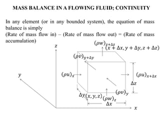
  • 1. In any element (or in any bounded system), the equation of mass balance is simply (Rate of mass flow in) – (Rate of mass flow out) = (Rate of mass accumulation) MASS BALANCE IN A FLOWING FLUID; CONTINUITY 𝜌𝑢 𝑥 𝜌𝑢 𝑥+∆𝑥 𝑥, 𝑦, 𝑧 𝑥 + ∆𝑥, 𝑦 + ∆𝑦, 𝑧 + ∆𝑧 ∆𝑥 ∆𝑧 ∆𝑦 𝑥 𝑧 𝑦 𝜌𝑤 𝑧 𝜌𝑤 𝑧+∆𝑧 𝜌𝑣 𝑦 𝜌𝑣 𝑦+∆𝑦
  • 2. Flux is defined as the rate of flow of any quantity per unit area. For a fluid of density 𝜌 in 𝑥 direction the mass flux in 𝑥 direction at the face 𝑥 is 𝜌𝑢 𝑥 ; the mass flux in 𝑥 direction at the face 𝑥+ ∆𝑥 is 𝜌𝑢 𝑥+∆𝑥; The rate of mass flow entering the element in 𝑥 direction 𝜌𝑢 𝑥 ∆𝑦∆𝑧 ; The rate of mass flow leaving the element in 𝑥 direction 𝜌𝑢 𝑥+∆𝑥∆𝑦∆𝑧; The rate of accumulation in the volume element is ∆𝑥∆𝑦∆𝑧 𝜕𝜌 𝜕𝑡 For a fluid of density 𝜌 in 𝑦 direction the mass flux in 𝑦 direction at the face 𝑦 is 𝜌𝑣 𝑦 ; the mass flux in 𝑦 direction at the face 𝑦+ ∆𝑦 is 𝜌𝑣 𝑦+∆𝑦; The rate of mass flow entering the element in 𝑦 direction 𝜌𝑣 𝑦 ∆𝑥∆𝑧 ; The rate of mass flow leaving the element in 𝑦 direction 𝜌𝑣 𝑦+∆𝑦∆𝑥∆𝑧; Similar terms can be obtained for a fluid in 𝑧 direction (𝑤 is velocity)
  • 3. 𝜌𝑢 𝑥 − 𝜌𝑢 𝑥+∆𝑥 ∆𝑦∆𝑧 + 𝜌𝑣 𝑦 − 𝜌𝑣 𝑦+∆𝑦 ∆𝑥∆𝑧 + 𝜌𝑤 𝑧 − 𝜌𝑤 𝑧+∆𝑧 ∆𝑥∆𝑦 = ∆𝑥∆𝑦∆𝑧 𝜕𝜌 𝜕𝑡 𝜌𝑢 𝑥 − 𝜌𝑢 𝑥+∆𝑥 ∆𝑥 + 𝜌𝑣 𝑦 − 𝜌𝑣 𝑦+∆𝑦 ∆𝑦 + 𝜌𝑤 𝑧 − 𝜌𝑤 𝑧+∆𝑧 ∆𝑧 = 𝜕𝜌 𝜕𝑡 𝜕𝜌 𝜕𝑡 = − 𝜕 𝜌𝑢 𝜕𝑥 + 𝜕 𝜌𝑣 𝜕𝑦 + 𝜕 𝜌𝑤 𝜕𝑧 = − ∇ ∙ 𝜌𝑉 The above equation is known as the equation of continuity. The quantity ∇ ∙ 𝜌𝑉 on the right hand side denotes the divergence of the mass velocity vector 𝜌𝑉. Taking the limit as ∆𝑥 , ∆𝑦 , and ∆𝑧 approach zero gives the differential equation of conservation of mass in a fluid. Dividing through ∆𝑥 ∆𝑦 ∆𝑧 gives.
  • 4. 𝜕𝜌 𝜕𝑡 = − 𝜌 𝜕𝑢 𝜕𝑥 + 𝑢 𝜕𝜌 𝜕𝑥 − 𝜌 𝜕𝑣 𝜕𝑦 + 𝑣 𝜕𝜌 𝜕𝑦 − 𝜌 𝜕𝑤 𝜕𝑧 + 𝑤 𝜕𝜌 𝜕𝑧 𝜕𝜌 𝜕𝑡 + 𝑢 𝜕𝜌 𝜕𝑥 + 𝑣 𝜕𝜌 𝜕𝑦 + 𝑤 𝜕𝜌 𝜕𝑧 = −𝜌 𝜕𝑢 𝜕𝑥 + 𝜕𝑣 𝜕𝑦 + 𝜕𝑤 𝜕𝑧 𝐷𝜌 𝐷𝑡 = −𝜌 𝜕𝑢 𝜕𝑥 + 𝜕𝑣 𝜕𝑦 + 𝜕𝑤 𝜕𝑧 = −𝜌 ∇ ∙ 𝑉 ∇ ∙ 𝑉 = 𝜕𝑢 𝜕𝑥 + 𝜕𝑣 𝜕𝑦 + 𝜕𝑤 𝜕𝑧 = 0 Continuity equation for a fluid with constant density. Often in engineering the fluid is almost incompressible and density may be considered constant Where Dρ/Dt is the substantial derivative or the derivative following the motion. At steady state 𝜕𝜌 𝜕𝑡 = 0. Carrying out the partial differentiation gives
  • 5. A stream line is an imaginary curve in a mass of flowing fluid so drawn that at every point on the curve, the net velocity vector is tangent to the stream line as shown in figure No net flow takes place across such a line. In turbulent flow, eddies do cross and recross a streamline, however, the net flow from such eddies is zero. One dimensional flow
  • 6. A stream tube, or stream filament, is a tube of any convenient cross- section and shape that is entirely bounded by stream lines. A stream tube can be visualized as an imaginary pipe in the mass of flowing fluid through the walls of which no net flow is occurring. If the tube has a differential cross-sectional area dS, the velocity through the tube can also be denoted by a single term u. The mass flow through the differential are is 𝑑𝑚 = 𝜌𝑢 𝑑𝑆 If the fluid is heated or cooled, the fluid density varies, but usually the variation is small and can be neglected.
  • 7. 𝑚 = 𝜌 𝑆 𝑢 𝑑𝑆 𝑉 ≡ 𝑚 𝜌𝑆 = 1 𝑆 𝑆 𝑢 𝑑𝑆 𝑉 = 𝑞 𝑆 The velocity 𝑉 also equals the volumetric flow rate divided by the cross-sectional area of the conduit It is also flux of volume or volume flux The average velocity 𝑉 of the entire stream flowing through a cross-sectional area S is defined by The flow rate through entire crosssection is
  • 8. 𝜌𝑏 𝑉𝑏 𝑆𝑏 𝑚 = 𝜌𝑎𝑆𝑎𝑉 𝑎= 𝜌𝑏𝑆𝑏𝑉𝑏 = 𝜌𝑆𝑉 𝑚 = 𝜋 4 𝐷𝑎 2𝜌𝑎𝑉 𝑎= 𝜋 4 𝐷𝑏 2 𝜌𝑏𝑉𝑏 𝜌𝑎𝑉 𝑎 𝐷𝑎 2 = 𝜌𝑏𝑉𝑏𝐷𝑏 2 𝜌𝑎𝑉𝑎 𝜌𝑏𝑉𝑏 = 𝐷𝑏 𝐷𝑎 2 𝑉𝑎 𝑉𝑏 = 𝐷𝑏 𝐷𝑎 2 Shell balance for mass flow Consider the system as shown in the figure below 𝑆𝑎 𝑉 𝑎 𝜌𝑎 Flow through circular cross section At steady state mass flow in is equal to mass flow out and the continuity equation becomes If density remains constant than Shell balance is
  • 9. 𝐺 ≡ 𝑚 𝑆 = 𝑉𝜌 Mass velocity In practice the mass velocity is expressed as kilograms per square meter per second, pounds per square foot per second. The advantage of using G is that it is independent of temperature and pressure when flow is steady (constant 𝑚) and the cross section is unchanged (Constant S). This fact is useful when compressible fluids are considered, for both 𝑉 and 𝜌 vary with temperature and pressure. The mass velocity G can also be described as mass current density or mass flux.
  • 10. A momentum balance may be made on a volume element in much the same way as a mass balance, but since velocity is a vector, the derivation is considerably complicated. The basic concept of the momentum balance is as follows DIFFERENTIAL MOMENTUM BALANCE; EQUATIONS OF MOTION Rate of momentum accumulation = Rate of momentum leaving sum of forces acting on the system + - The fluid is flowing through all six faces of the volume element in any arbitrary direction. Since velocity is a vector, Equation 1 has components in each of coordinate direction x,y, and z. First we consider only the x component of each term in Equation 1, the y and z components may be treated analogously. Rate of momentum entering
  • 11. 𝜌𝑢𝑢 𝑥 𝜌𝑢𝑢 𝑥+∆𝑥 𝑥, 𝑦, 𝑧 𝑥 + ∆𝑥, 𝑦 + ∆𝑦, 𝑧 + ∆𝑧 ∆𝑥 ∆𝑧 ∆𝑦 𝑥 𝑧 𝑦 𝜌𝑤𝑢 𝑧 𝜌𝑤𝑢 𝑧+∆𝑧 𝜌𝑣𝑢 𝑦 𝜌𝑣𝑢 𝑦+∆𝑦
  • 12. For a fluid of density 𝜌 in 𝑥 direction The rate at which the x component of momentum enters the face at x by convection is 𝜌𝑢𝑢 𝑥 ∆𝑦∆𝑧 ; The rate at which it leaves at 𝑥+ ∆𝑥 is 𝜌𝑢𝑢 𝑥+∆𝑥∆𝑦∆𝑧; The rate at which the x component of momentum enters the face at x by convection is 𝜌𝑤𝑢 𝑧 ∆𝑥∆𝑦 ; The rate at which it leaves at 𝑧+ ∆𝑧 is 𝜌𝑤𝑢 𝑧+∆𝑧∆𝑥∆𝑦; The rate at which the x component of momentum enters the face at y by convection is 𝜌𝑣𝑢 𝑦 ∆𝑥∆𝑧 ; The rate at which it leaves at 𝑦+ ∆𝑦 is 𝜌𝑣𝑢 𝑦+∆𝑦∆𝑥∆𝑧;
  • 13. Department of Chemical Engineering, AU College of Engineering (A) The rate of accumulation of momentum in the volume element is ∆𝑥∆𝑦∆𝑧 𝜕 𝜕𝑡 𝜌𝑢 𝜌𝑢𝑢 𝑥 − 𝜌𝑢𝑢 𝑥+∆𝑥 ∆𝑦∆𝑧 + 𝜌𝑣𝑢 𝑦 − 𝜌𝑣𝑢 𝑦+∆𝑦 ∆𝑥∆𝑧 + 𝜌𝑤𝑢 𝑧 − 𝜌𝑤𝑢 𝑧+∆𝑧 ∆𝑥∆𝑦 The net convective flow into the volume element is
  • 14. 𝜏𝑥𝑥 𝑥 𝜏𝑥𝑥 𝑥+∆𝑥 ∆𝑥 ∆𝑧 ∆𝑦 𝑥 𝑧 𝑦 𝜏𝑧𝑥 𝑧 𝜏𝑧𝑥 𝑧+∆𝑧 𝜏𝑦𝑥 𝑦 𝜏𝑦𝑥 𝑦+∆𝑦
  • 15. The rate at which the x component of momentum enters the face at x by molecular transport/Viscous forces is 𝜏𝑥𝑥 𝑥∆𝑦∆𝑧 and the rate at which it leaves at 𝑥 + ∆𝑥 is 𝜏𝑥𝑥 𝑥+∆𝑥∆𝑦∆𝑧 ; Considering x component in three directions x, y, and z The rate at which the x component of momentum enters the face at y by molecular transport/Viscous forces is 𝜏𝑦𝑥 𝑦 ∆𝑥∆𝑧 and the rate at which it leaves at 𝑦 + ∆𝑦 is 𝜏𝑦𝑥 𝑦+∆𝑦 ∆𝑥∆𝑧 ; The rate at which the x component of momentum enters the face at z by molecular transport/Viscous forces is 𝜏𝑧𝑥 𝑧∆𝑥∆𝑦 and the rate at which it leaves at 𝑧 + ∆𝑧 is 𝜏𝑧𝑥 𝑧+∆𝑧∆𝑥∆𝑦 ;
  • 16. 𝜏𝑥𝑥 𝑥 − 𝜏𝑥𝑥 𝑥+∆𝑥 ∆𝑦∆𝑧 + 𝜏𝑦𝑥 𝑦 − 𝜏𝑦𝑥 𝑦+∆𝑦 ∆𝑥∆𝑧 + 𝜏𝑧𝑥 𝑧 − 𝜏𝑧𝑥 𝑧+∆𝑧 ∆𝑥∆𝑦 Summing up these six contributions gives the net flow of x momentum into the volume element by viscous action: In most cases the important forces acting on the system arise from the fluid pressure 𝑝 and the gravitational force per unit mass g. the resultant of the forces in x direction is 𝑝 𝑥 − 𝑝 𝑥+∆𝑥 ∆𝑦∆𝑧 + ρ𝑔𝑥∆𝑥∆𝑦∆𝑧
  • 17. ∆𝑥∆𝑦∆𝑧 𝜕 𝜕𝑡 𝜌𝑢 = 𝜌𝑢𝑢 𝑥 − 𝜌𝑢𝑢 𝑥+∆𝑥 ∆𝑦∆𝑧 + 𝜌𝑣𝑢 𝑦 − 𝜌𝑣𝑢 𝑦+∆𝑦 ∆𝑥∆𝑧 + 𝜌𝑤𝑢 𝑧 − 𝜌𝑤𝑢 𝑧+∆𝑧 ∆𝑥∆𝑦 + 𝜏𝑥𝑥 𝑥 − 𝜏𝑥𝑥 𝑥+∆𝑥 ∆𝑦∆𝑧 + 𝜏𝑦𝑥 𝑦 − 𝜏𝑦𝑥 𝑦+∆𝑦 ∆𝑥∆𝑧 + 𝜏𝑧𝑥 𝑧 − 𝜏𝑧𝑥 𝑧+∆𝑧 ∆𝑥∆𝑦 + 𝑝 𝑥 − 𝑝 𝑥+∆𝑥 ∆𝑦∆𝑧 + ρ𝑔𝑥∆𝑥∆𝑦∆𝑧
  • 18. Dividing through ∆𝑥 ∆𝑦 ∆𝑧 Taking the limit as ∆𝑥 , ∆𝑦 , and ∆𝑧 approach zero gives the differential equation of momentum. 𝜕 𝜕𝑡 𝜌𝑢 = − 𝜕 𝜕𝑥 𝜌𝑢𝑢 + 𝜕 𝜕𝑦 𝜌𝑣𝑢 + 𝜕 𝜕𝑧 𝜌𝑤𝑢 − 𝜕 𝜕𝑥 𝜏𝑥𝑥 + 𝜕 𝜕𝑦 𝜏𝑦𝑥 + 𝜕 𝜕𝑧 𝜏𝑧𝑥 − 𝜕𝑝 𝜕𝑥 + 𝜌𝑔𝑥 𝜌 𝜕𝑢 𝜕𝑡 + 𝑢 𝜕𝜌 𝜕𝑡 = − 𝑢 𝜕 𝜕𝑥 𝜌𝑢 + 𝑢 𝜕 𝜕𝑦 𝜌𝑣 + 𝑢 𝜕 𝜕𝑧 𝜌𝑤 − 𝜌𝑢 𝜕𝑢 𝜕𝑥 + 𝜌𝑣 𝜕𝑢 𝜕𝑦 + 𝜌𝑤 𝜕𝑢 𝜕𝑧 − 𝜕 𝜕𝑥 𝜏𝑥𝑥 + 𝜕 𝜕𝑦 𝜏𝑦𝑥 + 𝜕 𝜕𝑧 𝜏𝑧𝑥 − 𝜕𝑝 𝜕𝑥 + 𝜌𝑔𝑥
  • 19. 𝜌 𝜕𝑢 𝜕𝑡 + 𝑢 𝜕𝜌 𝜕𝑡 = −𝑢 − 𝜕𝜌 𝜕𝑡 −𝜌 𝑢 𝜕𝑢 𝜕𝑥 + 𝑣 𝜕𝑢 𝜕𝑦 + 𝑤 𝜕𝑢 𝜕𝑧 − 𝜕 𝜕𝑥 𝜏𝑥𝑥 + 𝜕 𝜕𝑦 𝜏𝑦𝑥 + 𝜕 𝜕𝑧 𝜏𝑧𝑥 − 𝜕𝑝 𝜕𝑥 + 𝜌𝑔𝑥 𝜌 𝜕𝑢 𝜕𝑡 + 𝑢 𝜕𝑢 𝜕𝑥 + 𝑣 𝜕𝑢 𝜕𝑦 + 𝑤 𝜕𝑢 𝜕𝑧 = − 𝜕 𝜕𝑥 𝜏𝑥𝑥 + 𝜕 𝜕𝑦 𝜏𝑦𝑥 + 𝜕 𝜕𝑧 𝜏𝑧𝑥 − 𝜕𝑝 𝜕𝑥 + 𝜌𝑔𝑥 𝜌 𝐷𝑢 𝐷𝑡 = − 𝜕 𝜕𝑥 𝜏𝑥𝑥 + 𝜕 𝜕𝑦 𝜏𝑦𝑥 + 𝜕 𝜕𝑧 𝜏𝑧𝑥 − 𝜕𝑝 𝜕𝑥 + 𝜌𝑔𝑥
  • 20. 𝜌 𝐷𝑣 𝐷𝑡 = − 𝜕 𝜕𝑥 𝜏𝑥𝑦 + 𝜕 𝜕𝑦 𝜏𝑦𝑦 + 𝜕 𝜕𝑧 𝜏𝑧𝑦 − 𝜕𝑝 𝜕𝑦 + 𝜌𝑔𝑦 𝜌 𝐷𝑤 𝐷𝑡 = − 𝜕 𝜕𝑥 𝜏𝑥𝑧 + 𝜕 𝜕𝑦 𝜏𝑦𝑧 + 𝜕 𝜕𝑧 𝜏𝑧𝑧 − 𝜕𝑝 𝜕𝑧 + 𝜌𝑔𝑧 𝜌 𝐷𝑉 𝐷𝑡 = −∇𝑝 − ∇. 𝜏 + 𝜌𝑔
  • 21. 𝜏𝑥𝑥 = −2𝜇 𝜕𝑢 𝜕𝑥 + 2 3 𝜇 − 𝑘 ∇. 𝑉 𝜏𝑥𝑦 = 𝜏𝑦𝑥 = 𝜇 𝜕𝑢 𝜕𝑦 + 𝜕𝑣 𝜕𝑥 ∇. 𝑉 = 𝜕𝑢 𝜕𝑥 + 𝜕𝑣 𝜕𝑦 + 𝜕𝑤 𝜕𝑧 𝜌 𝐷𝑢 𝐷𝑡 = − 𝜕𝑝 𝜕𝑥 + 𝜕 𝜕𝑥 2𝜇 𝜕𝑢 𝜕𝑥 − 2 3 𝜇 − 𝑘 ∇. 𝑉 + 𝜕 𝜕𝑦 𝜇 𝜕𝑢 𝜕𝑦 + 𝜕𝑣 𝜕𝑥 + 𝜕 𝜕𝑧 𝜇 𝜕𝑤 𝜕𝑥 + 𝜕𝑢 𝜕𝑧 + 𝜌𝑔𝑥 𝜏𝑧𝑥 = 𝜏𝑥𝑧 = 𝜇 𝜕𝑤 𝜕𝑥 + 𝜕𝑢 𝜕𝑧 For Newtonian fluids the x direction components of stress tensor are Where k is the bulk viscosity. The general equations for a Newtonian fluid with varying density and viscosity are exemplified by the following equation for the x direction.
  • 22. 𝜏𝑥𝑦 = 𝜏𝑦𝑥 = 𝜇 𝜕𝑢 𝜕𝑦 + 𝜕𝑣 𝜕𝑥 ∇. 𝑉 = 𝜕𝑢 𝜕𝑥 + 𝜕𝑣 𝜕𝑦 + 𝜕𝑤 𝜕𝑧 𝜌 𝐷𝑣 𝐷𝑡 = − 𝜕𝑝 𝜕𝑦 + 𝜕 𝜕𝑥 𝜇 𝜕𝑢 𝜕𝑦 + 𝜕𝑣 𝜕𝑥 + 𝜕 𝜕𝑦 2𝜇 𝜕𝑣 𝜕𝑥 − 2 3 𝜇 − 𝑘 ∇. 𝑉 + 𝜕 𝜕𝑧 𝜇 𝜕𝑤 𝜕𝑦 + 𝜕𝑣 𝜕𝑧 + 𝜌𝑔𝑦 𝜏𝑦𝑧 = 𝜏𝑧𝑦 = 𝜇 𝜕𝑣 𝜕𝑧 + 𝜕𝑤 𝜕𝑦 𝜏𝑦𝑦 = −2𝜇 𝜕𝑣 𝜕𝑦 + 2 3 𝜇 − 𝑘 ∇. 𝑉
  • 23. ∇. 𝑉 = 𝜕𝑢 𝜕𝑥 + 𝜕𝑣 𝜕𝑦 + 𝜕𝑤 𝜕𝑧 𝜏𝑦𝑧 = 𝜏𝑧𝑦 = 𝜇 𝜕𝑣 𝜕𝑧 + 𝜕𝑤 𝜕𝑦 𝜏𝑧𝑥 = 𝜏𝑥𝑧 = 𝜇 𝜕𝑤 𝜕𝑥 + 𝜕𝑢 𝜕𝑧 𝜏𝑧𝑧 = −2𝜇 𝜕𝑤 𝜕𝑧 + 2 3 𝜇 − 𝑘 ∇. 𝑉 𝜌 𝐷𝑤 𝐷𝑡 = − 𝜕𝑝 𝜕𝑧 + 𝜕 𝜕𝑥 𝜇 𝜕𝑤 𝜕𝑥 + 𝜕𝑢 𝜕𝑧 + 𝜕 𝜕𝑦 𝜇 𝜕𝑤 𝜕𝑦 + 𝜕𝑣 𝜕𝑧 + 𝜕 𝜕𝑧 2𝜇 𝜕𝑣 𝜕𝑧 − 2 3 𝜇 − 𝑘 ∇. 𝑉 + 𝜌𝑔𝑧
  • 24. Navier Stokes equations. The previous equations are used in their complete form only in setting up highly complicated flow problems. In most situations restricted forms suffice. For a fluid of constant density and viscosity, the equations of motion, known as navier-stokes equations, are 𝜌 𝜕𝑢 𝜕𝑡 + 𝑢 𝜕𝑢 𝜕𝑥 + 𝑣 𝜕𝑢 𝜕𝑦 + 𝑤 𝜕𝑢 𝜕𝑧 = 𝜇 𝜕2𝑢 𝜕𝑥 + 𝜕2𝑢 𝜕𝑦 + 𝜕2𝑢 𝜕𝑧 − 𝜕𝑝 𝜕𝑥 + 𝜌𝑔𝑥 𝜌 𝜕𝑣 𝜕𝑡 + 𝑢 𝜕𝑣 𝜕𝑥 + 𝑣 𝜕𝑣 𝜕𝑦 + 𝑤 𝜕𝑣 𝜕𝑧 = 𝜇 𝜕2𝑣 𝜕𝑥 + 𝜕2𝑣 𝜕𝑦 + 𝜕2𝑣 𝜕𝑧 − 𝜕𝑝 𝜕𝑦 + 𝜌𝑔𝑦 𝜌 𝜕𝑤 𝜕𝑡 + 𝑢 𝜕𝑤 𝜕𝑥 + 𝑣 𝜕𝑤 𝜕𝑦 + 𝑤 𝜕𝑤 𝜕𝑧 = 𝜇 𝜕2𝑤 𝜕𝑥 + 𝜕2𝑤 𝜕𝑦 + 𝜕2𝑤 𝜕𝑧 − 𝜕𝑝 𝜕𝑧 + 𝜌𝑔𝑧
  • 25. In vector form these equations become 𝜌 𝐷𝑉 𝐷𝑡 = −∇𝑝 − 𝜇∇2 𝑽 + 𝜌𝒈 Euler’s equation. For constant density and zero viscosity, as in potential flow, the equation of motion known as Euler equation , is 𝜌 𝐷𝑉 𝐷𝑡 = −∇𝑝 + 𝜌𝒈 𝜌 𝜕𝑢 𝜕𝑡 + 𝑢 𝜕𝑢 𝜕𝑥 + 𝑣 𝜕𝑢 𝜕𝑦 + 𝑤 𝜕𝑢 𝜕𝑧 = − 𝜕𝑝 𝜕𝑥 + 𝜌𝑔𝑥
  • 26. 𝐹 = 𝑀𝑏 − 𝑀𝑎 MACROSCOPIC MOMENTUM BALANCES An overall momentum balance can be written for the control volume shown in figure, assuming that the flow is steady and unidirectional in the x direction. The sum of the forces acting on the fluid in the x direction equals the increase in the momentum flow rate of the fluid The momentum flow rate 𝑀 of a fluid stream having a mass flow rate 𝑚 and moving at a velocity u is 𝑚𝑢 . If u varies from point to point in the cross-section of the stream, however, the total momentum does not equal the product of mass flow rate and the average velocity, or 𝑚𝑉. In general some what greater than this.
  • 27. 𝑑𝑀 𝑑𝑆 = 𝜌𝑢 𝑢 = 𝜌𝑢2 𝑀 𝑆 = 𝜌 𝑆 𝑢2 𝑑𝑆 𝑆 𝛽 ≡ 𝑀 𝑆 𝜌𝑉2 The necessary correction factor is best found from the convective momentum flux. This is the product of the linear velocity normal to the cross section and the mass velocity(Mass Flux). For a differential cross sectional area dS, the momentum flux is The momentum flux of the whole stream, for constant density fluid, is The momentum correction factor is defined by 𝛽 = 𝜌 𝑆 𝑢2 𝑑𝑆 𝑆 𝜌𝑉2 = 1 𝑆 𝑆 𝑢 𝑉 2 𝑑𝑆
  • 28. 𝐹 = 𝑚 𝛽𝑏𝑉𝑏 − 𝛽𝑎𝑉 𝑎 𝐹 = 𝑝𝑎𝑆𝑎 − 𝑝𝑏𝑆𝑏 + 𝐹𝑤 − 𝐹 𝑔 𝑚 𝛽𝑏𝑉𝑏 − 𝛽𝑎𝑉 𝑎 = 𝑝𝑎𝑆𝑎 − 𝑝𝑏𝑆𝑏 + 𝐹𝑤 − 𝐹 𝑔 The modified momentum balance with correction factor is The forces acting on the system are 1. Pressure change in the direction of the flow 2. Shear stress at the boundary between fluid stream and the conduit 3. If the stream is inclined the appropriate component of force of gravity.
  • 29. 4.2. For a given fluid and a given distance between plates in a system like that shown in Figure 4.5. velocity 𝑣𝑜 must be large enough to counteract the effect of gravity; otherwise, some of the fluid will flow downward. In a particular system, the distance between plates is1 mm, and the fluid is an oil with a density of 900 kg/m3 and a viscosity of 50 mPa-s. The pressure drop 𝑑𝑝 𝑑𝑦 is negligible compared with the term 𝜌𝑔. (a) What is the minimum upward velocity of the moving plate so that all the fluid moves upward? (b) if 𝑣𝑜 is set at this minimum value, what is the fluid velocity midway between the plates? (c) What is the shear rate in the fluid at a stationary plate, at the moving plate, and midway between them? Use the equations in Example 4.3 Given Data Distance between plates = 1mm = 0.001 m Density of the oil ρ = 900 kg/m3 Viscosity of the oil 𝜇 = 50 mPa.S = 50 x 10-3 Pa-s
  • 30. (a) For none of the liquid to be flowing down dv/dx must be greater than or equal to zero at x=0. Also 𝜕𝑝 𝜕𝑦 can be neglected when compared with 𝜌𝑔. 𝜕𝑣 𝜕𝑥 − 𝑥 𝜇 𝜕𝑝 𝜕𝑦 + 𝜌𝑔 = 𝐶1 = 𝑣𝑜 𝐵 − 𝐵 2𝜇 𝜕𝑝 𝜕𝑦 + 𝜌𝑔 𝜕𝑣 𝜕𝑥 = 0 = 𝑣𝑜 𝐵 − 𝐵𝜌𝑔 2𝜇 𝑣𝑜 𝐵 = 𝐵𝜌𝑔 2𝜇 𝑣𝑜 = 𝐵2𝜌𝑔 2𝜇 = 0.00120.001900𝑥9.8065 2𝑥0.05 = 0.08826 𝑚 𝑠 = 88.26 𝑚𝑚/𝑠
  • 31. (b) The velocity at midway (x = B/2) is evaluated from the formula 𝑣 = 𝑣𝑜 𝑥 𝐵 − 1 2𝜇 𝜕𝑝 𝜕𝑦 + 𝜌𝑔 𝐵𝑥 − 𝑥2 𝑣 = 𝑣𝑜 𝐵 2𝐵 − 1 2𝜇 𝜌𝑔 𝐵 𝐵 2 − 𝐵 2 2 𝑣 = 𝑣𝑜 2 − 𝜌𝑔 2𝜇 𝐵2 4 𝑣 = 𝑣𝑜 2 − 𝑣𝑜 4 = 𝑣𝑜 4 = 0.08826 4 = 0.02206 𝑚 𝑠 = 22.06 𝑚𝑚/𝑠
  • 32. 4.9. The velocity profile in a fluid stream is approximated using a three part model, where the velocity is 1.6m/s in 15 percent cross- sectional area, 3.2m/s in 35 percent of the area, and 4.5m/s in the rest of the area. (a) How much does the total momentum of the fluid differ from the product of the mass flow rate and the average velocity? (b) Can you think of a situation where there is a velocity profile in the flow stream and the momentum flow is exactly equal to the mass flow times the average velocity? Given data Velocity of fluid for 15% 𝑉= 1.6 m/s Velocity of fluid for 15% 𝑉= 1.6 m/s Velocity of fluid for 35% 𝑉= 3.2 m/s Velocity of fluid for 50% 𝑉= 4.5 m/s
  • 33. Assume total cross-sectional area be S, Then Flow rate for 15 % area Q1 =1.6 x 0.15 =0.24S Flow rate for 35 % area Q2 =3.2 x 0.35 =1.12S Flow rate for 50 % area Q2 =4.5 x 0.50 =2.25S Total flow rate Q = 0.24S + 1.12S + 2.25S = 3.61S Average Velocity 𝑉 = Q/S = 3.61S/S = 3.61 m/s
  • 34. Momentum developed in 15 % area 𝑚1 𝜌 = 1.62𝑥0.15𝑆 = 0.384𝑆 Momentum developed in 35 % area 𝑚2 𝜌 = 3.22 𝑥0.35𝑆 = 3.584𝑆 Momentum developed in 50 % area 𝑚3 𝜌 = 4.52 𝑥0.50𝑆 = 10.125𝑆 Total momentum developed is 𝑚 𝜌 = 0.384𝑆 + 3.584𝑆 + 10.125𝑆 = 14.093𝑆 Total momentum based on average velocity 𝑚 𝜌 = 3.612 𝑆 = 13.0321𝑆 The ratio of momentum based on average velocity to actual Momentum 13.0321 14.093 = 0.9247
  • 35. The value of beta = 𝛽 = 14.093 13.0321 = 1.0814 The only situation where momentum is calculated from average velocity is in the plug flow region where velocity is same.
  • 36. 4.5. Water enters a 100-mm-ID 900 elbow, positioned in a horizontal plane, at a velocity of 6 m/s and a pressure of 70 kN/m2 gauge. Neglecting friction, what are the magnitude and the direction of the force that must be applied to the elbow to keep it in position without moving? Assume elbow is in the x-z plane with water entering in the x direction and leaving in the z direction. Since water flows horizontally Fg is 0. 𝑚 𝛽𝑏𝑉𝑏,𝑥 − 𝛽𝑎𝑉 𝑎,𝑥 = 𝑝𝑎𝑆𝑎,𝑥 − 𝑝𝑏𝑆𝑏,𝑥 + 𝐹𝑤,𝑥 𝑚 𝛽𝑏𝑉𝑏,𝑧 − 𝛽𝑎𝑉 𝑎,𝑧 = 𝑝𝑎𝑆𝑎,𝑧 − 𝑝𝑏𝑆𝑏,𝑧 + 𝐹𝑤,𝑧
  • 37. Given data Diameter of the pipe, D = 100 mm = 0.1 m Cross sectional area of pipe S = 𝜋 4 0.1 2 = 7.854 𝑥 10−3 m2 Velocity of water 𝑉= 6 m/s Pressure p = 70 kN/m2 = 70,000 N/m2 Mass flow rate 𝑚 = 1000 x 6 x 7.854 𝑥 10−3 = 47.1239 kg/s Density of water ρ= 1000 kg/m3
  • 38. Assume 𝛽𝑎 = 𝛽𝑏 = 1 𝑉 𝑎,𝑥 = 𝑉𝑏,𝑧 = 𝑉 = 6 𝑚/𝑠 𝑉𝑏,𝑥 = 𝑉 𝑎,𝑧 = 0 𝑚/𝑠 𝑆𝑎,𝑥 = 𝑆𝑏,𝑧 = 𝑆 = 7.854 𝑥 10−3 m2 𝑆𝑎,𝑧 = 𝑆𝑏,𝑥 = 0 𝑚2 𝐹𝑤,𝑥 = 𝑚 𝛽𝑏𝑉𝑏,𝑥 − 𝛽𝑎𝑉 𝑎,𝑥 − (𝑝𝑎𝑆𝑎,𝑥 − 𝑝𝑏𝑆𝑏,𝑥) 𝐹𝑤,𝑥 = 47.1239 0 − 6 − (70000𝑥0.007854 − 0) 𝐹𝑤,𝑥 = −832.5234 𝑁
  • 39. 𝐹𝑤,𝑧 = 𝑚 𝛽𝑏𝑉𝑏,𝑧 − 𝛽𝑎𝑉 𝑎,𝑧 − 𝑝𝑎𝑆𝑎,𝑧 − 𝑝𝑏𝑆𝑏,𝑧 𝐹𝑤,𝑧 = 47.1239 6 − 0 − 0 − 70000𝑥0.007854 𝐹𝑤,𝑧 = 832.5234 𝑁 832.5234 -832.5234 The total force of 832.5234√2 = 1177.3659 N will be acting in the direction shown
  • 40. Department of Chemical Engineering, AU College of Engineering (A) Layer flow with free surface 𝑚 𝛽𝑏𝑉𝑏 − 𝛽𝑎𝑉 𝑎 = 𝑝𝑎𝑆𝑎 − 𝑝𝑏𝑆𝑏 + 𝐹𝑤 − 𝐹 𝑔 0 Fg
  • 41. 𝐹 𝑔 cos ∅ − 𝜏𝐴 = 0 𝜏𝐿𝑏 = 𝜌𝑟𝐿𝑏𝑔 cos ∅ 𝜏 = 𝜌𝑟𝑔 cos ∅ 𝜏 = −𝜇 𝑑𝑢 𝑑𝑟 −𝜇 𝑑𝑢 𝑑𝑟 = 𝜌𝑟𝑔 cos ∅ 0 𝑢 𝑑𝑢 = − 𝜌𝑔 cos ∅ 𝜇 𝛿 𝑟 𝑟 𝑑𝑟
  • 42. 𝑢 = − 𝜌𝑔 cos ∅ 2𝜇 𝑟2 − 𝛿2 = 𝜌𝑔 cos ∅ 2𝜇 𝛿2 − 𝑟2 𝑚 = 0 𝛿 𝜌𝑢𝑏 𝑑𝑟 𝑚 𝑏 = 𝜌 0 𝛿 𝜌𝑔 cos ∅ 2𝜇 𝛿2 − 𝑟2 𝑑𝑟 𝑚 𝑏 = 𝜌2𝑔 cos ∅ 2𝜇 0 𝛿 𝛿2 − 𝑟2 𝑑𝑟 𝑚 𝑏 = 𝜌2𝑔 cos ∅ 2𝜇 𝛿3 − 𝛿3 3 𝑚 𝑏 = 𝜌 0 𝛿 𝑢 𝑑𝑟
  • 43. 𝑚 𝑏 = 𝛿3 𝜌2 𝑔 cos ∅ 3𝜇 = Г 𝛿3 = 3𝜇Г 𝜌2𝑔 cos ∅ 𝛿 = 3𝜇Г 𝜌2𝑔 cos ∅ 1 3
  • 44. 4.6. A vertical cylinder reactor 2.5 m in diameter and 4 m high is cooled by spraying water on the top and allowing the water to flow down the outside wall. The water flow rate is 0.15 m3/min, and the average water temperature is 40oC. Estimate the thickness of the layer of water. 𝛿 = 3𝜇Г 𝜌2𝑔 cos ∅ 1 3 = 3𝑥0.000656𝑥2.5 10002𝑥9.80665𝑥1 1 3 = 0.000399 = 0.4𝑚𝑚 Volumetric flow rate = 0.15/60 = 0.0025 m3/s Density of water = 1000 kg/m3 Viscosity of water = 0.656cP = 0.656x10⁻³ Pa-s Mass flow rate m = 0.0025 x 1000 = 2.5 kg/s b = (22/7) 2.5 = 7.857 m
  • 45. MECHANICAL ENERGY EQUATION Energy equation for potential flow; Bernoulli equation without friction The 𝑥 component of the Euler equation is 𝜌 𝜕𝑢 𝜕𝑡 + 𝑢 𝜕𝑢 𝜕𝑥 + 𝑣 𝜕𝑢 𝜕𝑦 + 𝑤 𝜕𝑢 𝜕𝑧 = − 𝜕𝑝 𝜕𝑥 + 𝜌𝑔𝑥
  • 46. Department of Chemical Engineering, AU College of Engineering (A) The unidirectional flow 𝑣 and 𝑤 are zero. Multiplying the remaining terms by the velocity u gives 𝜌𝑢 𝜕𝑢 𝜕𝑡 + 𝑢 𝜕𝑢 𝜕𝑥 = −𝑢 𝜕𝑝 𝜕𝑥 + 𝜌𝑢𝑔𝑥 𝜌 𝜕 𝑢2 2 𝜕𝑡 + 𝑢 𝜕 𝑢2 2 𝜕𝑥 = −𝑢 𝜕𝑝 𝜕𝑥 + 𝜌𝑢𝑔𝑥 This is the mechanical energy equation for unidirectional potential of fluids of constant density when flow rate varies with time.
  • 47. Consider now a volume element of a stream tube within a larger stream of fluid, as shown in figure flowing at steady flow. Assume the cross section of the tube increases continuously in the direction of flow and that the axis of tube is straight and inclined at an angle 𝝓 as shown.
  • 48. Since flow is steady 𝜕𝑢 𝜕𝑡 is zero. Since the flow is Unidirectional u is a function only of 𝑥. Since gravity acts in negative x direction 𝑔𝑥 = −𝑔 cos ∅ . And cos ∅ = dZ/dx 𝜌 𝜕𝑢 𝜕𝑡 + 𝑢 𝜕𝑢 𝜕𝑥 + 𝑣 𝜕𝑢 𝜕𝑦 + 𝑤 𝜕𝑢 𝜕𝑧 = − 𝜕𝑝 𝜕𝑥 + 𝜌𝑔𝑥 0 0 0 𝜌 𝑢 𝜕𝑢 𝜕𝑥 = − 𝜕𝑝 𝜕𝑥 − 𝜌𝑔 cos ∅ 𝜌 𝑑 𝑢2 2 𝑑𝑥 + 𝑑𝑝 𝑑𝑥 + 𝜌𝑔 𝑑𝑍 𝑑𝑥 = 0 𝑑 𝑢2 2 𝑑𝑥 + 1 𝜌 𝑑𝑝 𝑑𝑥 + 𝑔 𝑑𝑍 𝑑𝑥 = 0
  • 49. Integrating the equation we have 𝑝 𝜌 + 𝑔𝑍 + 𝑢2 2 = 𝑐𝑜𝑛𝑠𝑡 Integrating over the system shown in fiquare 𝑝𝑎 𝜌 + 𝑔𝑍𝑎 + 𝑢𝑎 2 2 = 𝑝𝑏 𝜌 + 𝑔𝑍𝑏 + 𝑢𝑏 2 2 Each term has a units of energy per unit mass 𝑔𝑍 represents Potential energy per unit mass
  • 50. 𝑢2 2 represents Kinetic energy per unit mass 𝑝 𝜌 represents Mechanical work done by forces external to the stream If velocity is reduced then either the datum height or pressure should increase or both should increase. Station a and b are chosen on the basis of convenience and are usall taken at locations where the most information about pressures, velocities, and heights are available.
  • 51. Bernoulli equation: correction for effects of solid boundaries. To extend the Bernoulli equation to cover the practical situations streams that are influenced by solid boundaries, two modifications are needed. The first is the correction of the kinetic energy term for variation of local velocity u with position in the boundary layer, The Second, of major importance , is the correction of equation for the existence of fluid friction, which appears whenever boundary layer forms.
  • 52. Kinetic energy of stream The term 𝑢2 2 is the kinetic energy of a unit mass of fluid all of which is flowing at the same velocity 𝑢. when the velocity varies across the stream cross section, the kinetic energy is found in the following manner. Consider a element of cross-sectional area 𝑑𝑆. The mass flow rate through this is 𝑢2 2 Each unit mass of flowing through area 𝑑𝑆 is therefore 𝑑𝐸𝑘 = 𝜌𝑢 𝑑𝑆 𝑢2 2 = 𝜌𝑢3 𝑑𝑆 2
  • 53. Consider a element of cross-sectional area 𝑑𝑆. The mass flow rate through this is 𝑢2 2 Each unit mass of flowing through area 𝑑𝑆 is therefore 𝐸𝑘 = 𝜌 2 𝑆 𝑢3 𝑑𝑆 𝐸𝑘 𝑚 = 𝜌 2 𝑆 𝑢3 𝑑𝑆 𝜌 𝑆 𝑢 𝑑𝑆 = 1 2 𝑆 𝑢3 𝑑𝑆 𝑉𝑆
  • 54. It is convenient to eliminate the integral by a factor operating on 𝑉2 2 to give the correct value of the kinetic energy 𝛼𝑉2 2 ≡ 𝐸𝑘 𝑚 = 𝑆 𝑢3 𝑑𝑆 2𝑉𝑆 𝛼 = 𝑆 𝑢3 𝑑𝑆 𝑉3𝑆 = 1 𝑆 𝑆 𝑢 𝑉 3 𝑑𝑆 𝛼 = 1 𝑆 𝑆 𝑢 𝑉 3 𝑑𝑆 𝛽 = 1 𝑆 𝑆 𝑢 𝑉 2 𝑑𝑆 𝑉 = 1 𝑆 𝑆 𝑢 𝑑𝑆
  • 55. Correction Bernoulli equation for fluid flow 𝑝𝑎 𝜌 + 𝑔𝑍𝑎 + 𝛼𝑎𝑉 𝑎 2 2 = 𝑝𝑏 𝜌 + 𝑔𝑍𝑏 + 𝛼𝑏𝑉𝑏 2 2 + ℎ𝑓 𝜂 = 𝑊 𝑝 − ℎ𝑓𝑝 𝑊 𝑝 Pump work in Bernoulli equation 𝑊 𝑝 − ℎ𝑓𝑝 ≡ 𝜂𝑊 𝑝
  • 56. 𝑝𝑎 𝜌 + 𝑔𝑍𝑎 + 𝛼𝑎𝑉 𝑎 2 2 + 𝝶𝑊 𝑝 = 𝑝𝑏 𝜌 + 𝑔𝑍𝑏 + 𝛼𝑏𝑉𝑏 2 2 + ℎ𝑓 Bernoulli equation with pump work and friction
  • 57. 4.3. Water at 200 C is pumped at a constant rate of 9 m3 /h from a large reservoir resting on the floor to the open top of an experimental absorption tower. The point of discharge is 5 m above the floor, and frictional losses in the 50-mm pipe from the reservoir to the tower amount to 2.5 J/kg. At what height in the reservoir must the water level be kept if the pump can develop only 0.1 k W? 5 M X X Za Given data Flow rate of water Q = 9 m3/hr Height Zb = 5m Diameter of pipe Db = 50 mm Frictional losses hf = 2.5 J/kg Pumping power P = 0.1 kW a b
  • 58. 5 M X X Za a b 𝑝𝑎 = 𝑝𝑏= 1 atm 𝑉𝑏 = 𝑄 𝑆𝑏 = 9 3600𝑥0.00196 = 1.276 𝑚/𝑠 𝑆𝑏 = 𝜋 4 𝐷𝑏 2 = 0.00196 𝑚2 Since 𝑉𝑏 is large in comparison with 𝑉 𝑎, 𝑉 𝑎 can be neglected 𝑚 = 𝑄𝜌 = 9 3600 𝑥998 = 2.495 𝑘𝑔/𝑠 𝝶𝑊 𝑝 = 𝑃 𝑚 = 0.1 𝑥1000 2.495 = 40.08 𝐽/𝑘𝑔 𝑎𝑠𝑠𝑢𝑚𝑒 𝞪𝑏 = 1
  • 59. 𝑝𝑎 𝜌 + 𝑔𝑍𝑎 + 𝛼𝑎𝑉 𝑎 2 2 + 𝝶𝑊 𝑝 = 𝑝𝑏 𝜌 + 𝑔𝑍𝑏 + 𝛼𝑏𝑉𝑏 2 2 + ℎ𝑓 𝑔𝑍𝑎 + 𝝶𝑊 𝑝 = 𝑔𝑍𝑏 + 𝛼𝑏𝑉𝑏 2 2 + ℎ𝑓 9.80665𝑍𝑎 + 40.08 = 9.80665𝑥5 + 1.2762 2 + 2.5 𝑍𝑎 = 12.267 9.80665 = 1.25 𝑚 9.80665𝑍𝑎 = 49.033 + 0.814 + 2.5 − 40.08 0 0
  • 60. 4.3. (a) A water tank is 30 ft in diameter and the normal depth is 25ft. The outlet is a 4-in. horizontal pipe at the bottom. If this pipe is sheared off close to the tank, what is the initial flow rate of water from the tank? (Neglect friction loss in the short stub of pipe.) (b) How long will it take for the tank to be empty? (c) calculate the average flow rate and compare it with the initial flow rate. Given data Diameter of tank Dtank = 30 ft = 30x0.3048 = 9.144 m Diameter of pipe Dpipe = 4 in = 4x0.0254 = 0.1016 m Height Za =0 m Height Zb = 25 ft = 25x0.3048 =7.62 m
  • 61. 30 ft 25 ft 𝑝𝑎 𝜌 + 𝑔𝑍𝑎 + 𝛼𝑎𝑉 𝑎 2 2 + 𝝶𝑊 𝑝 = 𝑝𝑏 𝜌 + 𝑔𝑍𝑏 + 𝛼𝑏𝑉𝑏 2 2 + ℎ𝑓 0 0 0 0 𝑔𝑍𝑎 = 𝛼𝑏𝑉𝑏 2 2 𝑉𝑏 2 = 2𝑔𝑍𝑎 𝑉𝑏 = 2𝑔𝑍𝑎 𝑉𝑏 = 2𝑥9.80665𝑥7.62 = 12.2251 𝑚/𝑠 Initial flow rate 𝑄 = 12.2251 𝑥 0.008107 = 0.099108 𝑚3/𝑠
  • 62. Volume of tank at any flow = Z Stank = 65.669 Z m3 Volume flow of tank = - dV/dt = - 65.669 dZ/dt 𝐴𝑙𝑠𝑜 𝑄 = 𝑆𝑝𝑖𝑝𝑒𝑢𝑏 = 𝑆𝑝𝑖𝑝𝑒 2𝑔𝑍 = 0.0359𝑍0.5 −65.669 𝑑𝑍 𝑑𝑡 = 0.0359𝑍0.5 𝑑𝑡 = − 65.669 0.0359 𝑍−0.5dZ 0 𝑡 𝑑𝑡 = −1829.22 7.62 0 𝑍−0.5 𝑑𝑍 𝑡 = −1829.22 𝑍0.5 0.5 7.62 0 = 1829.22 x 5.5209 = 10098 s = 2.81 hr
  • 63. Initial Volume of tank = Z Stank = 65.669x7.62 = 500.398 m3 Average flow rate = Q/t = 500.398/10098 = 0.4955 m3 /s This exactly half the initial flow rate.
  • 64. 4.8. A pump storage facility takes water from a river at night when demand is low and pumps it to a hilltop reservoir 500ft above the river. The water is returned through turbines in the daytime to help meet peak demand . (a) for two 30-inch pipes, each 2500 ft long and carrying 20000 gal/min, what pumping power is needed if the pump efficiency is 85 percent? The friction losses is estimated to be 15 ft of water. (b) How much power can be generated by the turbines using the same flow rate? (c) What is the overall efficiency of this installation as an energy storage system.