SlideShare une entreprise Scribd logo
1  sur  11
Télécharger pour lire hors ligne
Summary of current radiometric calibration coefficients for Landsat MSS, TM, ETM+,
and EO-1 ALI sensors
Gyanesh Chander a,
⁎, Brian L. Markham b
, Dennis L. Helder c
a
SGT, Inc.
1
contractor to the U.S. Geological Survey (USGS) Earth Resources Observation and Science (EROS) Center, Sioux Falls, SD 57198-0001, USA
b
National Aeronautics and Space Administration (NASA) Goddard Space Flight Center (GSFC), Greenbelt, MD 20771, USA
c
South Dakota State University (SDSU), Brookings, SD 57007, USA
a b s t r a c ta r t i c l e i n f o
Article history:
Received 10 December 2008
Received in revised form 16 January 2009
Accepted 17 January 2009
Keywords:
Landsat MSS, TM, ETM+
EO-1 ALI
Radiometric characterization & calibration
At-sensor spectral radiance
Top-of-atmosphere reflectance
At-sensor brightness temperature
This paper provides a summary of the current equations and rescaling factors for converting calibrated
Digital Numbers (DNs) to absolute units of at-sensor spectral radiance, Top-Of-Atmosphere (TOA)
reflectance, and at-sensor brightness temperature. It tabulates the necessary constants for the Multispectral
Scanner (MSS), Thematic Mapper (TM), Enhanced Thematic Mapper Plus (ETM+), and Advanced Land
Imager (ALI) sensors. These conversions provide a basis for standardized comparison of data in a single scene
or between images acquired on different dates or by different sensors. This paper forms a needed guide for
Landsat data users who now have access to the entire Landsat archive at no cost.
© 2009 Elsevier Inc. All rights reserved.
1. Introduction
The Landsat series of satellites provides the longest continuous record
of satellite-based observations. As such, Landsat is an invaluable resource
for monitoring global change and is a primary source of medium spatial
resolution Earth observations used in decision-making (Fuller et al.,1994;
Townshend et al.,1995; Goward & Williams,1997; Vogelmann et al., 2001;
Woodcock et al., 2001; Cohen & Goward, 2004; Goward et al., 2006;
Masek et al., 2008; Wulder et al., 2008). To meet observation require-
ments at a scale revealing both natural and human-induced landscape
changes, Landsat provides the only inventory of the global land surface
over time on a seasonal basis (Special issues on Landsat,1984,1985,1997,
2001, 2003, 2004, 2006). The Landsat Program began in early 1972 with
the launch of the first satellite in the series. As technological capabilities
increased, so did the amount and quality of image data captured by the
various sensors onboard the satellites. Table 1 presents general informa-
tion about each Landsat satellite.
Landsat satellites can be classified into three groups, based on
sensor and platform characteristics. The first group consists of Landsat
1 (L1), Landsat 2 (L2), and Landsat 3 (L3), with the Multispectral
Scanner (MSS) sensor and the Return Beam Vidicon (RBV) camera as
payloads on a “NIMBUS-like” platform. The spatial resolution of the
MSS sensor was approximately 79 m (but often processed to pixel size
of 60 m), with four bands ranging from the visible blue to the Near-
Infrared (NIR) wavelengths. The MSS sensor on L3 included a fifth
band in the thermal infrared wavelength, with a spectral range from
10.4 to 12.6 μm. The L1–L3 MSS sensors used a band-naming
convention of MSS-4, MSS-5, MSS-6, and MSS-7 for the blue, green,
red, and NIR bands, respectively (Markham & Barker, 1983). This
designation is obsolete, and to be consistent with the TM and ETM+
sensors, the MSS bands are referred to here as Bands 1–4, respectively.
The second group includes Landsat 4 (L4) and Landsat 5 (L5), which
carry the Thematic Mapper (TM) sensor, as well as the MSS, on the
Multimission Modular Spacecraft. This second generation of Landsat
satellites marked a significant advance in remote sensing through the
addition of a more sophisticated sensor, improved acquisition and
transmission of data, and more rapid data processing at a highly
automated processing facility. The MSS sensor was included to provide
continuity with the earlier Landsat missions, but TM data quickly
became the primary source of information used from these satellites
because the data offered enhanced spatial, spectral, radiometric, and
geometric performance over data from the MSS sensor. The TM sensor
has a spatial resolution of 30 m for the six reflective bands and 120 m for
the thermal band. Because there are no onboard recorders on these
sensors, acquisitions are limited to real-time downlink only.
The third group consists of Landsat 6 (L6) and Landsat 7 (L7),
which include the Enhanced Thematic Mapper (ETM) and the
Enhanced Thematic Mapper Plus (ETM+) sensors, respectively. No
MSS sensors were included on either satellite. Landsat 6 failed on
Remote Sensing of Environment 113 (2009) 893–903
⁎ Corresponding author. Tel.: +1 605 594 2554.
E-mail address: gchander@usgs.gov (G. Chander).
1
Work performed under USGS contract 08HQCN0005.
0034-4257/$ – see front matter © 2009 Elsevier Inc. All rights reserved.
doi:10.1016/j.rse.2009.01.007
Contents lists available at ScienceDirect
Remote Sensing of Environment
journal homepage: www.elsevier.com/locate/rse
launch. The L7 ETM+ sensor has a spatial resolution of 30 m for the six
reflective bands, 60 m for the thermal band, and includes a
panchromatic (pan) band with a 15 m resolution. L7 has a 378 gigabit
(Gb) Solid State Recorder (SSR) that can hold 42 min (approximately
100 scenes) of sensor data and 29 h of housekeeping telemetry
concurrently (L7 Science Data User's Handbook2
).
TheAdvanced Land Imager(ALI) onboard the Earth Observer-1(EO-1)
satellite is a technology demonstration that serves as a prototype for the
Landsat Data Continuity Mission (LDCM). The ALI observes the Earth in 10
spectral bands; nine spectral bands have a spatial resolution of 30 m, and a
pan band has a spatial resolution of 10 m.
The Landsat data archive at the U.S. Geological Survey (USGS) Earth
Resources Observation and Science(EROS) Centerholds an unequaled 36-
year record of the Earth's surface and is available at no cost to users via the
Internet (Woodcock et al., 2008). Users can access and search the Landsat
data archive via the EarthExplorer (EE)3
or Global Visualization Viewer
(GloVis)4
web sites. Note that the Landsat scenes collected by locations
within the International Ground Station (IGS) network may be available
only from the particular station that collected the scene.
2. Purpose
Equations and parameters to convert calibrated Digital Numbers
(DNs) to physical units, such as at-sensor radiance or Top-Of-Atmosphere
(TOA) reflectance, have been presented in a “sensor-specific” manner
elsewhere, e.g., MSS (Markham & Barker, 1986, 1987; Helder, 1993), TM
(Chander & Markham, 2003; Chander et al., 2007a), ETM+(Handbook2
),
and ALI (Markham et al., 2004a). This paper, however, tabulates the
necessary constants for all of the Landsat sensors in one place defined in a
consistent manner and provides a brief overview of the radiometric
calibration procedure summarizing the current accuracy of the at-sensor
spectral radiances obtained after performing these radiometric conver-
sions on standard data products generated by U.S. ground processing
systems.
3. Radiometric calibration procedure
The ability to detect and quantifychanges in the Earth's environment
depends on sensors that can provide calibrated (known accuracy and
precision) and consistent measurements of the Earth's surface features
through time. The correct interpretation of scientific information from a
global, long-term series of remote-sensing products requires the ability
to discriminate between product artifacts and changes in the Earth
processes being monitored (Roy et al., 2002). Radiometric characteriza-
tion and calibration is a prerequisite for creating high-quality science
data, and consequently, higher-level downstream products.
3.1. MSS sensors
Each MSS sensor incorporates an Internal Calibrator (IC) system,
consisting of a pair of lamp assemblies (for redundancy) and a rotating
shutter wheel. The shutter wheel includes a mirror and a neutral
density filter that varies in transmittance with rotation angle. The
calibration system output appears as a light pulse at the focal plane
that rises rapidly and then decays slowly. This pulse is referred to as
the calibration wedge (Markham & Barker, 1987). The radiometric
calibration of the MSS sensors is performed in two stages. First, raw
data from Bands 1–3 are “decompressed” or linearized and rescaled to
7 bits using fixed look-up tables. The look-up tables are derived from
prelaunch measurements of the compression amplifiers. Second, the
postlaunch gain and offset for each detector of all four bands are
individually calculated by a linear regression of the detector responses
to the samples of the in-orbit calibration wedge with the prelaunch
radiances for these samples. A reasonable estimate of the overall
calibration uncertainty of each MSS sensor at-sensor spectral
radiances is ±10%, which was the specified accuracy for the sensor
(Markham & Barker, 1987). In most cases, the ground processing
system must apply an additional step to uncalibrate the MSS data
because a number of MSS scenes were archived as radiometrically
corrected products. The previously calibrated archived MSS data must
be transformed back into raw DNs using the coefficients stored in the
data before applying the radiometric calibration procedure. Studies
are underway to evaluate the MSS calibration consistency and provide
post-calibration adjustments of the MSS sensors so they are consistent
over time and consistent between sensors (Helder, 2008).
3.2. TM sensors
The TM sensor includes an onboard calibration system called the
IC. The IC consists of a black shutter flag, three lamps, a cavity
blackbody, and the optical components necessary to get the lamp and
blackbody radiance to the focal plane. The lamps are used to calibrate
the reflective bands, and the blackbody is used to calibrate the thermal
band. Historically, the TM radiometric calibration procedure used the
detector's response to the IC to determine radiometric gains and
offsets on a scene-by-scene basis. Before launch, the effective radiance
of each lamp state for each reflective band's detector was determined
such that each detector's response to the internal lamp was compared
to its response to an external calibrated source. The reflective band
calibration algorithm for in-flight data used a regression of the
detector responses against the prelaunch radiances of the eight lamp
states. The slope of the regression represented the gain, while the
intercept represented the bias. This algorithm assumed that irradiance
of the calibration lamps remained constant over time since launch.
Any change in response was treated as a change in sensor response,
and thus was compensated for during processing. On-orbit data from
individual lamps indicated that the lamps were not particularly stable.
Because there was no way to validate the lamp radiances once in orbit,
the prelaunch measured radiances were the only metrics available for
2
http://landsathandbook.gsfc.nasa.gov/handbook.html.
3
http://earthexplorer.usgs.gov.
4
http://glovis.usgs.gov.
Table 1
General information about each Landsat satellite.
Satellite Sensors Launch date Decommission Altitude Inclination Period Repeat cycle Crossing
km degrees min days time (a.m.)
Landsat 1 MSS and RBV July 23, 1972 January 7, 1978 920 99.20 103.34 18 9:30
Landsat 2 MSS and RBV January 22, 1975 February 25, 1982 920 99.20 103.34 18 9:30
Landsat 3 MSS and RBV March 5, 1978 March 31, 1983 920 99.20 103.34 18 9:30
Landsat 4 MSS and TM July 16, 1982 June 30, 2001 705 98.20 98.20 16 9:45
Landsat 5 MSS and TM March 1, 1984 Operational 705 98.20 98.20 16 9:45
Landsat 6 ETM October 5, 1993 Did not achieve orbit
Landsat 7 ETM+ April 15, 1999 Operational 705 98.20 98.20 16 10:00
EO-1 ALI November 21, 2000 Operational 705 98.20 98.20 16 10:01
894 G. Chander et al. / Remote Sensing of Environment 113 (2009) 893–903
the regression procedure. Recent studies5
(Thome et al., 1997a, 1997b;
Helder et al., 1998; Markham et al., 1998; Teillet et al., 2001, 2004;
Chander et al., 2004a) indicate that the regression calibration did not
actually represent detector gains for most of the mission. However,
the regression procedure was used until 2003 to generate L5 TM data
products and is still used to generate L4 TM products. The calibration
uncertainties of the L4 TM at-sensor spectral radiances are ±10%,
which was the specified accuracy for the sensor (GSFC specification,
1981).
The L5 TM reflective band calibration procedure was updated in
2003 (Chander & Markham, 2003) to remove the dependence on the
changing IC lamps. The new calibration gains implemented on May 5,
2003, for the reflective bands (1–5, 7) were based on lifetime
radiometric calibration curves derived from the detectors' responses
to the IC, cross-calibration with ETM+, and vicarious measurements
(Chander et al., 2004a). The gains were further revised on April 2, 2007,
based on the detectors' responses to pseudo-invariant desert sites and
cross-calibration with ETM+ (Chander et al., 2007a). Although this
calibration update applies to all archived and future L5 TM data, the
principal improvements in the calibration are for data acquired during
the first eight years of the mission (1984–1991), where changes in the
sensor gain values are as much as 15%. The radiometric scaling
coefficients for Bands 1 and 2 for approximately the first eight years of
the mission have also been changed. Along with the revised reflective
band radiometric calibration on April 2, 2007, an sensor offset
correction of 0.092 W/(m2
sr μm), or about 0.68 K (at 300 K), was
added to all L5 TM thermal band (Band 6) data acquired since April
1999 (Barsi et al., 2007). The L5 TM radiometric calibration uncertainty
of the at-sensor spectral radiances is around 5% and is somewhat worse
for early years, when the sensor was changing more rapidly, and better
for later years (Helder et al., 2008). The L4 TM reflective bands and the
thermal band on both the TM sensors continue to be calibrated using
the IC. Further updates to improve the thermal band calibration are
being investigated, as is the calibration of the L4 TM.
3.3. ETM+ sensor
The ETM+ sensor has three onboard calibration devices for the
reflective bands: a Full Aperture Solar Calibrator (FASC), which is a
white painted diffuser panel; a Partial Aperture Solar Calibrator (PASC),
which is a set of optics that allows the ETM+ to image the Sun through
small holes; and an IC, which consists of two lamps, a blackbody, a
shutter, and optics to transfer the energy from the calibration sources to
the focal plane. The ETM+ sensor has also been calibrated vicariously
using Earth targets such as Railroad Valley (Thome, 2001; Thome et al.,
2004) and cross-calibrated with multiple sensors (Teillet et al., 2001,
2006, 2007; Thome et al., 2003; Chander et al., 2004b, 2007b, 2008).
The gain trends from the ETM+ sensor are regularly monitored on-
orbit using the onboard calibrators and vicarious calibration. The
calibration uncertainties of ETM+ at-sensor spectral radiances are
±5%. ETM+ is the most stable of the Landsat sensors, changing by no
more than 0.5% per year in its radiometric calibration (Markham et al.,
2004b). The ETM+ radiometric calibration procedure uses prelaunch
gain coefficients populated in the Calibration Parameter File (CPF).
These CPFs, issued quarterly, have both an “effective” and “version”
date. The effective date of the CPF must match the acquisition date of
the scene. A CPF version is active until a new CPF for that date period
supersedes it. Data can be processed with any version of a CPF; the later
versions have more refined parameters, as they reflect more data-rich
post-acquisition analysis.
The ETM+ images are acquired in either a low-or high-gain state.
The goal of using two gain settings is to maximize the sensors' 8-bit
radiometric resolution without saturating the detectors. For all bands,
5
Radiometric performance studies of the TM sensors have also led to a detailed
understanding of several image artifacts due to particular sensor characteristics
(Helder & Ruggles, 2004). These artifact corrections (such as Scan-Correlated Shift
[SCS], Memory Effect [ME], and Coherent Noise [CN]), along with detector-to-detector
normalization (Helder et al., 2004), are necessary to maintain the internal consistency
of the calibration within a scene.
Table 2
MSS spectral range, post-calibration dynamic ranges, and mean exoatmospheric solar irradiance (ESUNλ).
MSS sensors (Qcalmin =0 and Qcalmax =127)
Band Spectral range Center wavelength LMINλ LMAXλ Grescale Brescale ESUNλ
Units μm W/(m2
sr μm) (W/m2
sr μm)/DN W/(m2
sr μm) W/(m2
μm)
L1 MSS (NLAPS)
1 0.499–0.597 0.548 0 248 1.952760 0 1823
2 0.603–0.701 0.652 0 200 1.574800 0 1559
3 0.694–0.800 0.747 0 176 1.385830 0 1276
4 0.810–0.989 0.900 0 153 1.204720 0 880.1
L2 MSS (NLAPS)
1 0.497–0.598 0.548 8 263 2.007870 8 1829
2 0.607–0.710 0.659 6 176 1.338580 6 1539
3 0.697–0.802 0.750 6 152 1.149610 6 1268
4 0.807–0.990 0.899 3.66667 130.333 0.997373 3.66667 886.6
L3 MSS (NLAPS)
1 0.497–0.593 0.545 4 259 2.007870 4 1839
2 0.606–0.705 0.656 3 179 1.385830 3 1555
3 0.693–0.793 0.743 3 149 1.149610 3 1291
4 0.812–0.979 0.896 1 128 1.000000 1 887.9
L4 MSS (NLAPS)
1 0.495–0.605 0.550 4 238 1.842520 4 1827
2 0.603–0.696 0.650 4 164 1.259840 4 1569
3 0.701–0.813 0.757 5 142 1.078740 5 1260
4 0.808–1.023 0.916 4 116 0.881890 4 866.4
L5 MSS (NLAPS)
1 0.497–0.607 0.552 3 268 2.086610 3 1824
2 0.603–0.697 0.650 3 179 1.385830 3 1570
3 0.704–0.814 0.759 5 148 1.125980 5 1249
4 0.809–1.036 0.923 3 123 0.944882 3 853.4
Note 1: In some cases, the header file may have different rescaling factors than provided here. In these cases, the user should use the header file information that comes with the
product. Table 1 (Markham & Barker,1986, 1987) provides a summary of the band-specific LMINλ and LMAXλ rescaling factors that have been used at different times and by different
systems for the ground processing of MSS data.
895G. Chander et al. / Remote Sensing of Environment 113 (2009) 893–903
the low-gain dynamic range is approximately 1.5 times the high-gain
dynamic range. Therefore, low-gain mode is used to image surfaces
with high brightness (higher dynamic range but low sensitivity), and
high-gain mode is used to image surfaces with low brightness (lower
dynamic range but high sensitivity).
All of the ETM+ acquisitions after May 31, 2003, have an anomaly
caused by the failure of the Scan Line Corrector (SLC), which
compensated for the forward motion of the spacecraft so that all the
scans were aligned parallel with each other. The images with data loss
are referred to as SLC-off images, whereas images collected prior to
Table 3
TM spectral range, post-calibration dynamic ranges, and mean exoatmospheric solar irradiance (ESUNλ).
Note 1: The Q calmin =0 for data processed using NLAPS. The Q calmin =1 for data processed using LPGS.
Note 2: The LMINλ is typically set to a small negative number, so a “zero radiance” target will be scaled to a small positive DN value, even in the presence of sensor noise (typically 1
DN or less [1 sigma]). This value is usually not changed throughout the mission.
Note 3: In mid-2009, the processing of L4 TM data will transition from NLAPS to LPGS. NLAPS used IC-based calibration. The L4 TM data processed by LPGS will be radiometrically calibrated
using a new lifetime gain model procedure and revised calibration parameters. Use the header file information that comes with the product and the above rescaling factors will not be
applicable. The numbers highlighted in grey are the revised (LMAXλ=163) post-calibration dynamic ranges for L4 TM Band 1 data acquired between July 16,1982 (launch), and August 23,1986.
Note 4: The radiometric scaling coefficients for L5 TM Bands 1 and 2 for approximately the first eight years (1984–1991) of the mission were changed to optimize the dynamic range and better
preserve the sensitivity of the early mission data. The numbers highlighted in grey are the revised (LMAXλ=169, 333) post-calibration dynamic ranges for L5 TM Band 1 and 2 data acquired
between March 1, 1984 (launch), and December 31, 1991 (Chander et al., 2007a).
Table 4
ETM+ spectral range, post-calibration dynamic ranges, and mean exoatmospheric solar irradiance (ESUNλ).
L7 ETM+ Sensor (Qcalmin =1 and Qcalmax =255)
Band Spectral range Center wavelength LMINλ LMAXλ Grescale Brescale ESUNλ
Units μm W/(m2
sr μm) (W/m2
sr μm)/DN W/(m2
sr μm) W/(m2
μm)
Low gain (LPGS)
1 0.452–0.514 0.483 −6.2 293.7 1.180709 −7.38 1997
2 0.519–0.601 0.560 −6.4 300.9 1.209843 −7.61 1812
3 0.631–0.692 0.662 −5.0 234.4 0.942520 −5.94 1533
4 0.772–0.898 0.835 −5.1 241.1 0.969291 −6.07 1039
5 1.547–1.748 1.648 −1.0 47.57 0.191220 −1.19 230.8
6 10.31–12.36 11.335 0.0 17.04 0.067087 −0.07 N/A
7 2.065–2.346 2.206 −0.35 16.54 0.066496 −0.42 84.90
PAN 0.515–0.896 0.706 −4.7 243.1 0.975591 −5.68 1362
High Gain (LPGS)
1 0.452–0.514 0.483 −6.2 191.6 0.778740 −6.98 1997
2 0.519–0.601 0.560 −6.4 196.5 0.798819 −7.20 1812
3 0.631–0.692 0.662 −5.0 152.9 0.621654 −5.62 1533
4 0.772–0.898 0.835 −5.1 157.4 0.639764 −5.74 1039
5 1.547–1.748 1.648 −1.0 31.06 0.126220 −1.13 230.8
6 10.31–12.36 11.335 3.2 12.65 0.037205 3.16 N/A
7 2.065–2.346 2.206 −0.35 10.80 0.043898 −0.39 84.90
PAN 0.515–0.896 0.706 −4.7 158.3 0.641732 −5.34 1362
896 G. Chander et al. / Remote Sensing of Environment 113 (2009) 893–903
the SLC failure are referred to as SLC-on images (i.e., no data gaps
exist). The malfunction of the SLC mirror assembly resulted in the loss
of approximately 22% of the normal scene area (Storey et al., 2005).
The missing data affects most of the image, with scan gaps varying in
width from one pixel or less near the center of the image to 14 pixels
along the east and west edges of the image, creating a repeating
wedge-shaped pattern along the edges. The middle of the scene,
approximately 22 km wide on a Level 1 product, contains very little
duplication or data loss. Note that the SLC failure has no impact on the
radiometric performance with the valid pixels.
3.4. ALI sensor
The ALI has two onboard radiometric calibration devices: a lamp-
based system and a solar-diffuser with variable irradiance controlled
by an aperture door. In addition to its onboard calibrators, ALI has the
ability to collect lunar and stellar observations for calibration
purposes. The ALI radiometric calibration procedure uses a fixed set
of detector-by-detector gains established shortly after launch and
biases measured shortly after each scene acquisition by closing the
ALI's shutter. The calibration uncertainties of the ALI at-sensor spectral
radiances are ±5% (Mendenhall & Lencioni, 2002). The ALI sensor is
well-behaved and stable, with changes in the response being less than
2% per year even early in the mission, and averaging, at most, slightly
more than 1% per year over the full mission (Markham et al., 2006).
4. Conversion to at-sensor spectral radiance (Qcal-to-Lλ)
Calculation of at-sensor spectral radiance is the fundamental step
in converting image data from multiple sensors and platforms into a
physically meaningful common radiometric scale. Radiometric cali-
bration of the MSS, TM, ETM+, and ALI sensors involves rescaling the
raw digital numbers (Q) transmitted from the satellite to calibrated
digital numbers (Qcal)6
, which have the same radiometric scaling for
all scenes processed on the ground for a specific period.
During radiometric calibration, pixel values (Q) from raw,
unprocessed image data are converted to units of absolute spectral
radiance using 32-bit floating-point calculations. The absolute
radiance values are then scaled to 7-bit (MSS, Qcalmax = 127), 8-bit
(TM and ETM+, Qcalmax = 255), and 16-bit (ALI, Qcalmax = 32767)
numbers representing Qcal before output to distribution media.
Conversion from Qcal in Level 1 products back to at-sensor spectral
radiance (Lλ) requires knowledge of the lower and upper limit of the
original rescaling factors. The following equation is used to perform
the Qcal-to-Lλ conversion for Level 1 products:
Lλ =
LMAXλ − LMINλ
Qcalmax − Qcalmin
 
Qcal − Qcalminð Þ + LMINλ
or
Lλ = Grescale × Qcal + Brescale
where :
Grescale =
LMAXλ − LMINλ
Qcalmax − Qcalmin
Brescale = LMINλ −
LMAXλ − LMINλ
Qcalmax − Qcalmin
 
Qcalmin
ð1Þ
where
Lλ= Spectral radiance at the sensor's aperture [W/(m2
sr μm)]
Qcal= Quantized calibrated pixel value [DN]
Qcalmin= Minimum quantized calibrated pixel value corresponding
to LMINλ [DN]
Qcalmax= Maximum quantized calibrated pixel value corresponding
to LMAXλ [DN]
LMINλ= Spectral at-sensor radiance that is scaled to Qcalmin [W/(m2
sr μm)]
LMAXλ= Spectral at-sensor radiance that is scaled to Qcalmax [W/(m2
sr μm)]
Grescale= Band-specific rescaling gain factor [(W/(m2
sr μm))/DN]
Brescale= Band-specific rescaling bias factor [W/(m2
sr μm)]
Historically, the MSS and TM calibration information is presented in
spectral radiance units of mW/(cm2
sr μm). To maintain consistency with
ETM+ spectral radiance, units of W/(m2
sr μm) are now used for MSS and
TM calibration information. The conversion factor is 1:10 when converting
from mW/(cm2
sr μm) units to W/(m2
sr μm). Tables 2, 3, 4, and 5
summarize the spectral range, post-calibration dynamic ranges7
(LMINλ
and LMAXλ scaling parameters and the corresponding rescaling gain
[Grescale] and rescaling bias [Brescale] values), and mean exoatmospheric
solar irradiance (ESUNλ) for the MSS, TM, ETM+, and ALI sensors,
respectively.
6
These are the DNs that users receive with Level 1 Landsat products.
7
The post-calibration dynamic ranges summarized in Tables 2–5 are only applicable
to Landsat data processed and distributed by the USGS EROS Center. The IGSs may
process the data differently, and these rescaling factors may not be applicable. “Special
collections,” such as the Multi-Resolution Land Characteristics Consortium (MRLC) or
Global Land Survey (GLS), may have a different processing history, so the user needs to
verify the respective product header information.
Table 5
ALI spectral range, post-calibration dynamic ranges, and mean exoatmospheric solar irradiance (ESUNλ).
EO-1 ALI Sensor (Qcalmin =1 and Qcalmax =32767)
Band Spectral range Center wavelength LMINλ LMAXλ Grescale Brescale ESUNλ
Units μm W/(m2
sr μm) (W/m2
sr μm)/DN W/(m2
sr μm) W/(m2
μm)
PAN 0.480–0.690 0.585 −2.18 784.2 0.024 −2.2 1724
1P 0.433–0.453 0.443 −3.36 1471 0.045 −3.4 1857
1 0.450–0.515 0.483 −4.36 1405 0.043 −4.4 1996
2 0.525–0.605 0.565 −1.87 915.5 0.028 −1.9 1807
3 0.633–0.690 0.662 −1.28 588.5 0.018 −1.3 1536
4 0.775–0.805 0.790 −0.84 359.6 0.011 −0.85 1145
4P 0.845–0.890 0.868 −0.641 297.5 0.0091 −0.65 955.8
5P 1.200–1.300 1.250 −1.29 270.7 0.0083 −1.3 452.3
5 1.550–1.750 1.650 −0.597 91.14 0.0028 −0.6 235.1
7 2.080–2.350 2.215 −0.209 29.61 0.00091 −0.21 82.38
All EO-1 ALI standard Level 1 products are processed through the EO-1 Product Generation System (EPGS).
897G. Chander et al. / Remote Sensing of Environment 113 (2009) 893–903
Tables 2–5 give the prelaunch “measured” (as-built performance)
spectral ranges. These numbers are slightly different from the original
filter specification. The center wavelengths are the average of the two
spectral range numbers. Figs.1 and 2 show the Relative Spectral Response
(RSR) profiles of the Landsat MSS (Markham  Barker, 1983), TM
(Markham  Barker, 1985), ETM+(Handbook2
), and ALI (Mendenhall 
Parker, 1999) sensors measured during prelaunch characterization. The
ETM+ spectral bands were designed to mimic the standard TM spectral
bands 1–7. The ALI bands were designed to mimic the six standard ETM+
solar reflective spectral bands 1–5, and 7; three new bands,1p, 4p, and 5p,
were added to more effectively address atmospheric interference effects
and specific applications. The ALI band numbering corresponds with the
ETM+ spectral bands. Bands not present on the ETM+ sensor are given
the “p,” or prime, designation. MSS spectral bands are significantly
different from TM and ETM+ spectral bands.
The post-calibration dynamic ranges are band-specific rescaling
factors typically provided in the Level 1 product header file. Over
the life of the Landsat sensors, occasional changes have occurred in
Fig. 1. Comparison of the solar reflective bands RSR profiles of L1–5 MSS sensors.
898 G. Chander et al. / Remote Sensing of Environment 113 (2009) 893–903
the post-calibration dynamic range. Future changes are anticipated,
especially in the MSS and TM data, because of the possible
adjustment of the calibration constants based on comparisons to
absolute radiometric measurements made on the ground. In some
cases, the header file may have different rescaling factors than
provided in the table included here. In these cases, the user should
use the header file information that comes with the product.
Two processing systems will continue to generate Landsat data
products: the Level 1 Product Generation System (LPGS) and the
National Land Archive Production System (NLAPS). Starting December
8, 2008, all L7 ETM+ and L5 TM (except Thematic Mapper-Archive
[TM-A]8
products) standard Level 1 products are processed through
the LPGS, and all L4 TM and MSS standard Level 1 products are
processed through the NLAPS. The Landsat Program is working toward
transitioning the processing of all Landsat data to LPGS (Kline, personal
8
A small number of TM scenes were archived as radiometrically corrected products
known as TM-A data. The TM-A data are archived on a scene-by-scene basis (instead of
intervals). The L4 and L5 TM-A scenes will continue to be processed using NLAPS (with
Qcalmin =0), which attempts to uncalibrate the previously applied calibration and
generates the product using updated calibration procedures. Note that approximately
80 L4 TM and approximately 13,300 L5 TM scenes are archived as TM-A data, with
acquisition dates ranging between Sept.1982 and Aug. 1990.
Fig. 2. Comparison of the solar reflective bands RSR profiles of L4 TM, L5 TM, L7 ETM+, and EO-1 ALI sensors.
899G. Chander et al. / Remote Sensing of Environment 113 (2009) 893–903
communication). In mid-2009, the processing of L4 TM data will
transition from NLAPS to LPGS. The scenes processed using LPGS include
a header file (.MTL), which lists the LMINλ and LMAXλ values but not the
rescaling gain and bias numbers. The scenes processed using NLAPS
include a processing history work order report (.WO), which lists the
rescaling gain and bias numbers but not the LMINλ and LMAXλ.
The sensitivity of the detector changes over time, causing a change in
the detector gain applied during radiometric calibration. However, the
numbers presented in Tables 2–5 are the rescaling factors, which are the
post-calibration dynamic ranges. The LMINλ and LMAXλ are a repre-
sentation of how the output Landsat Level 1 data products are scaled in
at-sensor radiance units. Generally, there is no need to change the LMINλ
or LMAXλ unless something changes drastically on the sensor. Thus,
there is notime dependence for any of the rescaling factors inTables 2–5.
5. Conversion to TOA reflectance (Lλ-to-ρP)
A reduction in scene-to-scene variability can be achieved by
converting the at-sensor spectral radiance to exoatmospheric TOA
reflectance, also known as in-band planetary albedo. When comparing
images from different sensors, there are three advantages to using TOA
reflectance instead of at-sensor spectral radiance. First, it removes the
cosine effect of different solar zenith angles due to the time difference
between data acquisitions. Second, TOA reflectance compensates for
different values of the exoatmospheric solar irradiance arising from
spectral band differences. Third, the TOA reflectance corrects for the
variation in the Earth–Sun distance between different data acquisition
dates. These variations can be significant geographically and temporally.
The TOA reflectance of the Earth is computed according to the equation:
ρλ =
π Á Lλ Á d2
ESUNλ Á cos θs
ð2Þ
where
ρλ= Planetary TOA reflectance [unitless]
π= Mathematical constant equal to ~3.14159 [unitless]
Lλ= Spectral radiance at the sensor's aperture [W/(m2
sr μm)]
d= Earth–Sun distance [astronomical units]
ESUNλ= Mean exoatmospheric solar irradiance [W/(m2
μm)]
θs= Solar zenith angle [degrees9
]
Note that the cosine of the solar zenith angle is equal to the sine of
the solar elevation angle. The solar elevation angle at the Landsat
scene center is typically stored in the Level 1 product header file (.MTL
or .WO) or retrieved from the USGS EarthExplorer or GloVis online
interfaces under the respective scene metadata (these web sites also
contain the acquisition time in hours, minutes, and seconds). The TOA
reflectance calculation requires the Earth–Sun distance (d). Table 6
presents d in astronomical units throughout a year generated using
the Jet Propulsion Laboratory (JPL) Ephemeris10
(DE405) data. The d
numbers are also tabulated in the Nautical Almanac Office.
The last column of Tables 2–5 summarizes solar exoatmospheric
spectral irradiances (ESUNλ) for the MSS, TM, ETM+, and ALI sensors
using the Thuillier solar spectrum (Thuillier et al., 2003). The Committee
on Earth Observation Satellites (CEOS) Working Group on Calibration and
Validation (WGCV) recommends11
using this spectrum for applications in
optical-based Earth Observation that use an exoatmospheric solar
irradiance spectrum. The Thuillier spectrum is believed to be the most
accurate and an improvement over the other solar spectrum. Note that the
CHKUR solar spectrum in MODTRAN 4.0 (Air Force Laboratory,1998) was
used previously for ETM+(Handbook2
) and TM (Chander  Markham,
2003), whereas the Neckel and Lab (Neckel  Labs,1984) and Iqbal (Iqbal,
1983) solar spectrums were used for MSS and TM solar irradiance values
(MarkhamBarker,1986).Theprimarydifferences occurin Bands5 and7.
For comparisons to other sensors, users need to verify that the same solar
spectrum is used for all sensors.
6. Conversion to at-sensor brightness temperature (Lλ-to-T)
The thermal band data (Band 6 onTM and ETM+) can be converted
from at-sensor spectral radiance to effective at-sensor brightness
temperature. The at-sensor brightness temperature assumes that the
Earth's surface is a black body (i.e., spectral emissivity is 1), and
includes atmospheric effects (absorption and emissions along path).
The at-sensor temperature uses the prelaunch calibration constants
given in Table 7. The conversion formula from the at-sensor's spectral
radiance to at-sensor brightness temperature is:
T =
K2
ln K1
Lλ
+ 1
  ð3Þ
where:
T= Effective at-sensor brightness temperature [K]
K2= Calibration constant 2 [K]
Fig. 2 (continued).
9
Note that Excel, Matlab, C, and many other software applications use radians, not
degrees, to perform calculations. The conversion from degrees to radians is a
multiplication factor of pi/180.
10
http://ssd.jpl.nasa.gov/?horizons.
11
CEOS-recommended solar irradiance spectrum, http://wgcv.ceos.org.
900 G. Chander et al. / Remote Sensing of Environment 113 (2009) 893–903
K1= Calibration constant 1 [W/(m2
sr μm)]
Lλ= Spectral radiance at the sensor's aperture [W/(m2
sr μm)]
ln= Natural logarithm
The ETM+ Level 1 product has two thermal bands, one acquired
using a low gain setting (often referred to as Band 6 L; useful
temperature range of 130–350 K) and the other using a high gain
setting (often referred to as Band 6H; useful temperature range of
240–320 K). The noise equivalent change in temperature (NEΔT) at
280 K for ETM+ high gain is 0.22 and for low gain is 0.28. The TM Level
1 product has only one thermal band (there is no gain setting on the
TM sensor), and the thermal band images have a useful temperature
Table 6
Earth–Sun distance (d) in astronomical units for Day of the Year (DOY).
DOY d DOY d DOY d DOY d DOY d DOY d
1 0.98331 61 0.99108 121 1.00756 181 1.01665 241 1.00992 301 0.99359
2 0.98330 62 0.99133 122 1.00781 182 1.01667 242 1.00969 302 0.99332
3 0.98330 63 0.99158 123 1.00806 183 1.01668 243 1.00946 303 0.99306
4 0.98330 64 0.99183 124 1.00831 184 1.01670 244 1.00922 304 0.99279
5 0.98330 65 0.99208 125 1.00856 185 1.01670 245 1.00898 305 0.99253
6 0.98332 66 0.99234 126 1.00880 186 1.01670 246 1.00874 306 0.99228
7 0.98333 67 0.99260 127 1.00904 187 1.01670 247 1.00850 307 0.99202
8 0.98335 68 0.99286 128 1.00928 188 1.01669 248 1.00825 308 0.99177
9 0.98338 69 0.99312 129 1.00952 189 1.01668 249 1.00800 309 0.99152
10 0.98341 70 0.99339 130 1.00975 190 1.01666 250 1.00775 310 0.99127
11 0.98345 71 0.99365 131 1.00998 191 1.01664 251 1.00750 311 0.99102
12 0.98349 72 0.99392 132 1.01020 192 1.01661 252 1.00724 312 0.99078
13 0.98354 73 0.99419 133 1.01043 193 1.01658 253 1.00698 313 0.99054
14 0.98359 74 0.99446 134 1.01065 194 1.01655 254 1.00672 314 0.99030
15 0.98365 75 0.99474 135 1.01087 195 1.01650 255 1.00646 315 0.99007
16 0.98371 76 0.99501 136 1.01108 196 1.01646 256 1.00620 316 0.98983
17 0.98378 77 0.99529 137 1.01129 197 1.01641 257 1.00593 317 0.98961
18 0.98385 78 0.99556 138 1.01150 198 1.01635 258 1.00566 318 0.98938
19 0.98393 79 0.99584 139 1.01170 199 1.01629 259 1.00539 319 0.98916
20 0.98401 80 0.99612 140 1.01191 200 1.01623 260 1.00512 320 0.98894
21 0.98410 81 0.99640 141 1.01210 201 1.01616 261 1.00485 321 0.98872
22 0.98419 82 0.99669 142 1.01230 202 1.01609 262 1.00457 322 0.98851
23 0.98428 83 0.99697 143 1.01249 203 1.01601 263 1.00430 323 0.98830
24 0.98439 84 0.99725 144 1.01267 204 1.01592 264 1.00402 324 0.98809
25 0.98449 85 0.99754 145 1.01286 205 1.01584 265 1.00374 325 0.98789
26 0.98460 86 0.99782 146 1.01304 206 1.01575 266 1.00346 326 0.98769
27 0.98472 87 0.99811 147 1.01321 207 1.01565 267 1.00318 327 0.98750
28 0.98484 88 0.99840 148 1.01338 208 1.01555 268 1.00290 328 0.98731
29 0.98496 89 0.99868 149 1.01355 209 1.01544 269 1.00262 329 0.98712
30 0.98509 90 0.99897 150 1.01371 210 1.01533 270 1.00234 330 0.98694
31 0.98523 91 0.99926 151 1.01387 211 1.01522 271 1.00205 331 0.98676
32 0.98536 92 0.99954 152 1.01403 212 1.01510 272 1.00177 332 0.98658
33 0.98551 93 0.99983 153 1.01418 213 1.01497 273 1.00148 333 0.98641
34 0.98565 94 1.00012 154 1.01433 214 1.01485 274 1.00119 334 0.98624
35 0.98580 95 1.00041 155 1.01447 215 1.01471 275 1.00091 335 0.98608
36 0.98596 96 1.00069 156 1.01461 216 1.01458 276 1.00062 336 0.98592
37 0.98612 97 1.00098 157 1.01475 217 1.01444 277 1.00033 337 0.98577
38 0.98628 98 1.00127 158 1.01488 218 1.01429 278 1.00005 338 0.98562
39 0.98645 99 1.00155 159 1.01500 219 1.01414 279 0.99976 339 0.98547
40 0.98662 100 1.00184 160 1.01513 220 1.01399 280 0.99947 340 0.98533
41 0.98680 101 1.00212 161 1.01524 221 1.01383 281 0.99918 341 0.98519
42 0.98698 102 1.00240 162 1.01536 222 1.01367 282 0.99890 342 0.98506
43 0.98717 103 1.00269 163 1.01547 223 1.01351 283 0.99861 343 0.98493
44 0.98735 104 1.00297 164 1.01557 224 1.01334 284 0.99832 344 0.98481
45 0.98755 105 1.00325 165 1.01567 225 1.01317 285 0.99804 345 0.98469
46 0.98774 106 1.00353 166 1.01577 226 1.01299 286 0.99775 346 0.98457
47 0.98794 107 1.00381 167 1.01586 227 1.01281 287 0.99747 347 0.98446
48 0.98814 108 1.00409 168 1.01595 228 1.01263 288 0.99718 348 0.98436
49 0.98835 109 1.00437 169 1.01603 229 1.01244 289 0.99690 349 0.98426
50 0.98856 110 1.00464 170 1.01610 230 1.01225 290 0.99662 350 0.98416
51 0.98877 111 1.00492 171 1.01618 231 1.01205 291 0.99634 351 0.98407
52 0.98899 112 1.00519 172 1.01625 232 1.01186 292 0.99605 352 0.98399
53 0.98921 113 1.00546 173 1.01631 233 1.01165 293 0.99577 353 0.98391
54 0.98944 114 1.00573 174 1.01637 234 1.01145 294 0.99550 354 0.98383
55 0.98966 115 1.00600 175 1.01642 235 1.01124 295 0.99522 355 0.98376
56 0.98989 116 1.00626 176 1.01647 236 1.01103 296 0.99494 356 0.98370
57 0.99012 117 1.00653 177 1.01652 237 1.01081 297 0.99467 357 0.98363
58 0.99036 118 1.00679 178 1.01656 238 1.01060 298 0.99440 358 0.98358
59 0.99060 119 1.00705 179 1.01659 239 1.01037 299 0.99412 359 0.98353
60 0.99084 120 1.00731 180 1.01662 240 1.01015 300 0.99385 360 0.98348
361 0.98344
362 0.98340
363 0.98337
364 0.98335
365 0.98333
366 0.98331
901G. Chander et al. / Remote Sensing of Environment 113 (2009) 893–903
range of 200–340 K. The NEΔT at 280 K for L5 TM is 0.17–0.30 (Barsi
et al., 2003).
7. Conclusion
This paper provides equations and rescaling factors for converting
Landsat calibrated DNs to absolute units of at-sensor spectral radiance,
TOA reflectance, and at-sensor brightness temperature. It tabulates the
necessary constants for the MSS, TM, ETM+, and ALI sensors in a
coherent manner using the same units and definitions. This paper forms
a needed guide for Landsat data users who now have access to the entire
Landsat archive at no cost. Studies are ongoing to evaluate the MSS
calibration consistency and provide post-calibration adjustments of the
MSS sensors so they are consistent over time and consistent between
sensors. Further updates to improve the TM and ETM+ thermal band
calibration are being investigated, as is the calibration of the L4 TM.
Acknowledgments
This work was partially supported by the NASA Land-Cover and
Land-Use Change (LCLUC) Grant NNH08AI30I. The authors acknowl-
edge the support of David Aaron (SDSU) for digitizing the spectral
responses for the MSS sensors and Julia Barsi (SSAI) for generating the
Earth–Sun distance. Special thanks are extended to a number of
colleagues for reviewing drafts of this manuscript. The anonymous
reviewers' comments were particularly valuable and their efforts are
greatly appreciated. Any use of trade, product, or firm names is for
descriptive purposes only and does not imply endorsement by the U.S.
Government.
Appendix A
References
Air Force Research Laboratory (1998). Modtran Users Manual, Versions 3.7 and 4.0 : Hanscom
Air Force Base, MA.
Barsi, J. A., Schott, J. R., Palluconi, F. D., Helder, D. L., Hook, S. J., Markham, B. L., Chander,
G.,  O'Donnell, E. M. (2003). Landsat TM and ETM+ thermal band calibration.
Canadian Journal of Remote Sensing, 29(2), 141−153.
Barsi, J. A., Hook, S. J., Schott, J. R., Raqueno, N. G.,  Markham, B. L. (2007). Landsat-5
Thematic Mapper thermal band calibration update. IEEE Transactions on Geoscience
and Remote Sensing, 44, 552−555.
Chander, G.,  Markham, B. L. (2003). Revised Landsat-5 TM radiometric calibration
procedures, and post-calibration dynamic ranges. IEEE Transactions on Geoscience
and Remote Sensing, 41, 2674−2677.
Chander, G., Helder, D. L., Markham, B. L., Dewald, J., Kaita, E., Thome, K. J., Micijevic, E., 
Ruggles, T. (2004a). Landsat 5 TM on-orbit absolute radiometric performance. IEEE
Transactions on Geoscience and Remote Sensing, 42, 2747−2760.
Chander, G., Meyer, D. J.,  Helder, D. L. (2004b). Cross-calibration of the Landsat-7 ETM+
and EO-1 ALI sensors. IEEE Transactions on Geoscience and Remote Sensing, 42(12),
2821−2831.
Chander, G., Markham, B. L.,  Barsi, J. A. (2007a). Revised Landsat 5 Thematic Mapper
radiometric calibration.IEEE Transactions on Geoscience and Remote Sensing,44, 490−494.
Chander, G., Angal, A., Choi, T., Meyer, D. J., Xiong, X.,  Teillet, P. M. (2007b). Cross-
calibration of the Terra MODIS, Landsat-7 ETM+ and EO-1 ALI sensors using near
simultaneous surface observation over Railroad Valley Playa, Nevada test site. In J. J.
Butler  J. Xiong (Eds.), Proceedings of SPIE Conference 6677 on Earth Observing
Systems XII, SPIE, Vol. 6677. (pp. 66770Y: 1−12) San Diego, CA.
Chander, G., Coan, M. J.,  Scaramuzza, P. L. (2008). Evaluation and comparison of the
IRS-P6 and the Landsat Sensors. IEEE Transactions on Geoscience and Remote Sensing,
46(1), 209−221.
Cohen, W. B.,  Goward, S. N. (2004). Landsat's role in ecological applications of remote
sensing. BioScience, 54(6), 535−545.
Fuller, R. M., Groom, G. B.,  Jones, A. R. (1994). The land cover map of Great Britain: An
automated classification of Landsat Thematic Mapper data. Photogrammetric
Engineering and Remote Sensing, 60, 553−562.
Goward, S. N.,  Williams, D. L. (1997). Landsat and Earth Systems Science: Development of
terrestrial monitoring.Photogrammetric Engineering and Remote Sensing,63(7), 887−900.
Goward, S., Irons, J., Franks, S., Arvidson, T., Williams, D.,  Faundeen, J. (2006). Historical
record of Landsat global coverage: Mission operations, NSLRSDA, and international
cooperator stations. Photogrammetric Engineering and Remote Sensing, 72, 1155−1169.
GSFC Specification for the Thematic Mapper System and Associated Test Equipment.
(Rev C., January 1981) GSFC 400-8-D-210C, NASA, Goddard Space Flight Center,
Greenbelt, MD.
Helder, D. L. (1993). MSS radiometric calibration handbook. Report to the U.S. Geological
Survey (USGS) Earth Resources Observation and Science (EROS) Center.
Helder, D. L., Boncyk, W. C.,  Morfitt, R. (1998). Absolute calibration of the Landsat Thematic
Mapper using the internal calibrator. Proc. IGARSS, Seattle, WA, 1998 (pp. 2716−2718).
Helder, D. L. (2008a). Consistent radiometric calibration of the historical Landsat
archive. Proceedings of PECORA Denver, Colorado.
Helder, D. L., Markham, B. L., Thome, K. J., Barsi, J. A., Chander, G.,  Malla, R. (2008b).
Updated radiometric calibration for the Landsat 5 Thematic Mapper reflective
bands. IEEE Transactions on Geoscience and Remote Sensing, 46(10), 3309−3325.
Helder, D.L.,  Ruggles, T. A. (2004a). Landsat ThematicMapper reflectiveband radiometric
artifacts. IEEE Transactions on Geoscience and Remote Sensing, 44, 2704−2716.
Helder, D. L., Ruggles, T. A., Dewald, J. D.,  Madhavan, S. (2004b). Landsat-5 Thematic
Mapper reflective-band radiometric stability. IEEE Transactions on Geoscience and
Remote Sensing, 44, 2704−2716.
Iqbal, M. (1983). Introduction to solar radiation. New York: Academic Press.
Markham, B. L.,  Barker, J. L. (1983). Spectral characterization of the Landsat-4 MSS
sensors. Photogrammetric Engineering and Remote Sensing, 49(6), 811−833.
Markham, B. L.,  Barker, J. L. (1985). Spectral characterization of the LANDSAT
Thematic Mapper sensors'. International Journal of Remote Sensing, 6(5), 697−716.
Markham, B. L.,  Barker, J. L. (1986). Landsat MSS and TM post-calibration dynamic
ranges, exoatmospheric reflectances and at-satellite temperatures. Earth Observa-
tion Satellite Co., Lanham, MD, Landsat Tech. Note 1.
Markham, B. L.,  Barker, J. L. (1987). Radiometric properties of U.S. processed Landsat
MSS Data. Remote Sensing of Environment, 22, 39−71.
Markham, B. L., Seiferth, J. C., Smid, J.,  Barker, J. L. (1998). Lifetime responsivity
behavior of the Landsat-5 Thematic Mapper. Proceedings of SPIE Conference 3427 on
Earth Observing Systems, SPIE, Vol. 3427. (pp. 420−431) San Diego, CA.
Markham, B. L., Chander, G., Morfitt, R., Hollaren, D., Mendenhall, J. F.,  Ong, L. (2004a).
Radiometric processing and calibration of EO-1 Advanced Land Imager data. Proceedings
of PECORA 16 “Global Priorities in Land Remote Sensing” South Dakota: Sioux Falls.
Table A1
To maintain consistency, all Landsat scenes are based on the following naming convention.
Format Example:
LXSPPPRRRYYYYDDDGSIVV
L=Landsat
Sensor Examples:
LM10170391976031AAA01(MSS)
LT40170361982320XXX08 (TM)
LE70160392004262EDC02 (ETM+)X=Sensor
S=Satellite
PPP = Worldwide Reference
System (WRS) Path
RRR=WRS Row
YYYY=Year
DDD=Day of Year
GSI=Ground Station Identifier ⁎
VV=Version
⁎Ground Stations Identifiers-Data received at these sites are held at EROS
AAA=North American site
unknown
GNC=Gatineau, Canada
ASA=Alice Springs, Australia LGS=EROS, SD, USA, Landsat 5 data acquired by
EROS beginning July 1, 2001FUI=Fucino, Italy (Historical)
GLC=Gilmore Creek, AK, US MOR=Moscow, Russia
HOA=Hobart, Australia MLK=Malinda, Kenya
KIS=Kiruna, Sweden IKR=Irkutsk, Russia
MTI=Matera, Italy CHM=Chetumal, Mexico
EDC=Receiving site unknown XXO=Receiving site unknown
PAC=Prince Albert, Canada XXX=Receiving site unknown
Table A2
Standard Level 1 product specifications.
Product Type – Level 1T (Terrain Corrected)
Pixel Size – 15/30/60 meters
Output format – GeoTIFF
Resampling Method – Cubic Convolution (CC)
Map Projection – Universal Transverse Mercator (UTM)
Polar Stereographic for Antarctica
Image Orientation – Map (North Up)
Distribution – File Transfer Protocol (FTP) Download only
Table 7
TM and ETM+ thermal band calibration constants.
Constant K1 K2
Units W/(m2
sr μm) Kelvin
L4 TM 671.62 1284.30
L5 TM 607.76 1260.56
L7 ETM+ 666.09 1282.71
902 G. Chander et al. / Remote Sensing of Environment 113 (2009) 893–903
Markham, B. L., Thome, K., Barsi, J., Kaita, E., Helder, D., Barker, J.,  Scaramuzza, P. (2004b).
Landsat-7 ETM+ On-Orbit reflective-band radiometric stability and absolute calibra-
tion. IEEE Transactions on Geoscience and Remote Sensing, 42, 2810−2820.
Markham, B. L., Ong, L., Barsi, J. A., Mendenhall, J. A., Lencioni, D. E., Helder, D. L.,
Hollaren, D. H.,  Morfitt, R. M. (2006). Radiometric calibration stability of the EO-1
Advanced Land Imager: 5 Years on-orbit. In R. Meynart, S. P. Neeck,  H. Shimoda
(Eds.), Proceedings of SPIE Conference 6361 on Sensors, Systems, and Next-Generation
Satellites X, SPIE, Vol. 6361. (pp. 66770U: 1−12) San Diego, CA.
Masek, J. G., Vermote, Huang, C., Wolfe, R., Cohen, W., Hall, F., Kutler, J.,  Nelson, P.
(2008). North American forest disturbance mapped from a decadal Landsat record.
Remote Sensing of Environment, 112, 2914−2926.
Mendenhall, J. A.,  Parker, A. C. (1999). Spectral calibration of the EO-1 Advanced Land
Imager. Proceedings of SPIE Conference 3750 on Earth Observing Systems IV, SPIE, Vol.
3750. (pp. 109−116) Denver, Colorado.
Mendenhall, J. A.,  Lencioni, D.E. (2002). EO-1 advanced land imageron-orbit radiometric
calibration. International Geoscience and Remote Sensing Symposium Toronto, Canada.
Nautical Almanac Office. The Nautical Almanac for the Year (United States Naval
Observatory) (Washington, DC: U.S. Government Printing Office).
Neckel, H.,  Labs, D. (1984). The solar radiation between 3300 and 12500 A. Solar
Physics, 90, 205.
Roy, D., Borak, J., Devadiga, S., Wolfe, R., Zheng, M.,  Descloitres, J. (2002). The MODIS land
product quality assessment approach. Remote Sensing of Environment, 83, 62−76.
Special Issue on Landsat 4 (1984). IEEE Transactions on Geoscience and Remote Sensing,
GE-22(3), 160 51(9). Guest Editor: Solomonson, V.V.
Special Issue on Landsat Image Data Quality Analysis (LIDQA) (1985). Photogrammetric
Engineering and Remote Sensing, 51(9) Guest Editors: Markham, B.L., and Barker, J.L.
Special Issue on 25th Anniversary of Landsat (1997). Photogrammetric Engineering and
Remote Sensing, 63(7) Guest Editor: Salomonson, V.V.
Special Issue on Landsat 7 (2001). Remote Sensing of Environment, 78(1–2), 1−220
Guest Editors: Goward, S.N., and Masek, J.G.
Special Issue on Synergistic Utilization of Landsat 7 (2003). Canadian Journal of Remote
Sensing, 29(2), 141−297 Guest Editor: Teillet, P.M.
Special Issue on Landsat Sensor Performance Characterization (2004). IEEE Transactions
on Geoscience and Remote Sensing, 42(12), 2687−2855 Guest Editors: Markham, B.L.,
Storey, J.C., Crawford, M.M., Goodenough, D.G., Irons, J.R.
Special Issue on Landsat Operations: Past, Present and Future (2006). Photogrammetric
Engineering and Remote Sensing, 72(10) Guest Editors: Williams, D.L, Goward, S.N.,
Arvidson, T.
Storey, J. C., Scaramuzza, P.,  Schmidt, G. (2005). Landsat 7 scan line corrector-off gap
filled product development. PECORA 16 Conference Proceedings, Sioux Falls, South
Dakota (pp. 23−27).
Teillet, P. M., Barker, J. L., Markham, B. L., Irish, R. R., Fedosejeves, G.,  Storey, J. C. (2001).
Radiometric cross-calibration of the Landsat-7 ETM+ and Landsat-5 TM sensors
based on tandem data sets. Remote Sensing of Environment, 78(1–2), 39−54.
Teillet, P. M., Helder, D. L., Ruggles, T. A., Landry, R., Ahern, F. J., Higgs, N. J., et al. (2004). A
definitive calibration record for the Landsat-5 Thematic Mapper anchored to the
Landsat-7 radiometric scale. Canadian Journal of Remote Sensing, 30(4), 631−643.
Teillet, P. M., Markham, B. L.,  Irish, R. R. (2006). Landsat cross-calibration based on near
simultaneous imaging of common ground targets. Remote Sensing of Environment, 102
(3–4), 264−270.
Teillet, P. M., Fedosejevs, G., Thome, K. J.,  Barker, J. L. (2007). Impacts of spectral band
difference effects on radiometric cross-calibration between satellite sensors in the
solar-reflective spectral domain. Remote Sensing of Environment, 110, 393−409.
Thome, K. J. (2001). Absolute radiometric calibration of Landsat 7 ETM+ using the
reflectance-based method. Remote Sensing of Environment, 78(1–2), 27−38.
Thome, K. J., Markham, B. L., Barker, J. L., Slater, P. L.,  Biggar, S. (1997a). Radiometric
calibration of Landsat. Photogrammetric Engineering and Remote Sensing, 63, 853−858.
Thome, K. J., Crowther, B. G.,  Biggar, S. F. (1997b). Reflectance- and irradiance-based
calibration of Landsat-5 Thematic Mapper. Canadian Journal of Remote Sensing, 23,
309−317.
Thome, K. J., Biggar, S. F.,  Wisniewski, W. (2003). Cross comparison of EO-1 sensors
and other earth resources sensors to Landsat-7 ETM+ using Railroad Valley Playa.
IEEE Transactions on Geoscience and Remote Sensing, 41, 1180−1188.
Thome, K. J., Helder, D. L., Aaron, D. A.,  Dewald, J. (2004). Landsat 5 TM and Landsat-7
ETM+ absolute radiometric calibration using reflectance based method. IEEE
Transactions on Geoscience and Remote Sensing, 42(12), 2777−2785.
Thuillier, G., Herse, M., Labs, S., Foujols, T., Peetermans, W., Gillotay, D., Simon, P. C., 
Mandel, H. (2003). The solar spectral irradiance from 200 to 2400 nm as measured
by SOLSPEC Spectrometer from the ATLAS 123 and EURECA missions.Solar Physics,
214(1), 1−22 Solar Physics.
Townshend, J. R. G., Bell, V., Desch, A. C., Havlicek, C., Justice, C. O., Lawrence, W. E., Skole,
D., Chomentowski, W. W., Moore, B., Salas, W.,  Tucjer, C. J. (1995). The NASA
Landsat Pathfinder Humid Tropical Deforestation Project. Proceedings Land Satellite
Information in the Next Decade, ASPRS Conference (pp. 76−87). Vienna, Virginia.
Vogelmann, J. E., Howard, S. M., Yang, L., Larson, C. R., Wylie, B. K.,  Van Driel, J. N.
(2001). Completion of the 1990's National Land Cover Data Set for the
conterminous United States. Photogrammetric Engineering and Remote Sensing, 67,
650−662.
Woodcock, C. E., Macomber, S. A., Pax-Lenney, M.,  Cohen, W. C. (2001). Monitoring
large areas for forest change using Landsat: Generalization across space, time and
Landsat sensors. Remote Sensing of Environment, 78, 194−203.
Woodcock, C. E., Allen, A. A., Anderson, M., Belward, A. S., Bindschadler, R., Cohen, W. B.,
Gao, F., Goward, S. N., Helder, D., Helmer, E., Nemani, R., Oreapoulos, L., Schott, J.,
Thenkabail, P. S., Vermote, E. F., Vogelmann, J., Wulder, M. A.,  Wynne, R. (2008). Free
access to Landsat imagery. Science, 320, 1011.
Wulder, M. A., White, J. C., Goward, S. N., Masek, J. G., Irons, J. R., Herold, M., Cohen, W. B.,
Loveland, T. R.,  Woodcock, C. E. (2008). Landsat continuity: Issues and opportunities
for land cover monitoring. Remote Sensing of Environment, 112, 955−969.
903G. Chander et al. / Remote Sensing of Environment 113 (2009) 893–903

Contenu connexe

Tendances

Rahul seminar2 2_for_slideshare.pptx
Rahul seminar2 2_for_slideshare.pptxRahul seminar2 2_for_slideshare.pptx
Rahul seminar2 2_for_slideshare.pptxRahulSingh769902
 
Remote Sensing and its Applications in Agriculture
Remote Sensing and its Applications in AgricultureRemote Sensing and its Applications in Agriculture
Remote Sensing and its Applications in AgricultureVikas Kashyap
 
Remote Sensing Vivek
Remote Sensing VivekRemote Sensing Vivek
Remote Sensing Vivekvivek akkala
 
Fundamentals of Remote Sensing- A training module
Fundamentals of Remote Sensing- A training moduleFundamentals of Remote Sensing- A training module
Fundamentals of Remote Sensing- A training moduleNishant Sinha
 
Aerial photography vs RS satellite
Aerial photography vs RS satelliteAerial photography vs RS satellite
Aerial photography vs RS satelliteSumant Diwakar
 
Sensors for remote sensing
Sensors for remote sensingSensors for remote sensing
Sensors for remote sensingMohsin Siddique
 
Satellite image Processing Seminar Report
Satellite image Processing Seminar ReportSatellite image Processing Seminar Report
Satellite image Processing Seminar Reportalok ray
 
Hyperspectral remote sensing for oil exploration
Hyperspectral remote sensing for oil explorationHyperspectral remote sensing for oil exploration
Hyperspectral remote sensing for oil explorationJayanth Joshua
 
Remote Sensing and its Application
Remote Sensing and its ApplicationRemote Sensing and its Application
Remote Sensing and its ApplicationRashmi Yadav
 
Application of remote sensing in forest ecosystem
Application of remote sensing in forest ecosystemApplication of remote sensing in forest ecosystem
Application of remote sensing in forest ecosystemaliya nasir
 
Remote Sensing - A tool of plant disease management
Remote Sensing - A tool of plant disease managementRemote Sensing - A tool of plant disease management
Remote Sensing - A tool of plant disease managementAnand Choudhary
 
Remote sensing in Plants
Remote sensing in PlantsRemote sensing in Plants
Remote sensing in PlantsBasimAnees
 
HYPERSPECTRAL RS IN MINERAL MAPPING
HYPERSPECTRAL RS IN MINERAL MAPPINGHYPERSPECTRAL RS IN MINERAL MAPPING
HYPERSPECTRAL RS IN MINERAL MAPPINGAbhiram Kanigolla
 
Sensor Network for Landslide Monitoring With Laser Ranging System Avoiding Ra...
Sensor Network for Landslide Monitoring With Laser Ranging System Avoiding Ra...Sensor Network for Landslide Monitoring With Laser Ranging System Avoiding Ra...
Sensor Network for Landslide Monitoring With Laser Ranging System Avoiding Ra...Waqas Tariq
 
thenkabail-uav-germany-final1b
thenkabail-uav-germany-final1bthenkabail-uav-germany-final1b
thenkabail-uav-germany-final1bPrasad Thenkabail
 
Landslide monitoring systems & techniques
Landslide monitoring systems & techniquesLandslide monitoring systems & techniques
Landslide monitoring systems & techniquesmaneeb
 
hyperspectral remote sensing and its geological applications
hyperspectral remote sensing and its geological applicationshyperspectral remote sensing and its geological applications
hyperspectral remote sensing and its geological applicationsabhijeet_banerjee
 
Assessing stress by using remote sensing
Assessing stress by using remote sensingAssessing stress by using remote sensing
Assessing stress by using remote sensingChongtham Allaylay Devi
 

Tendances (20)

Rahul seminar2 2_for_slideshare.pptx
Rahul seminar2 2_for_slideshare.pptxRahul seminar2 2_for_slideshare.pptx
Rahul seminar2 2_for_slideshare.pptx
 
Remote Sensing and its Applications in Agriculture
Remote Sensing and its Applications in AgricultureRemote Sensing and its Applications in Agriculture
Remote Sensing and its Applications in Agriculture
 
Remote Sensing Vivek
Remote Sensing VivekRemote Sensing Vivek
Remote Sensing Vivek
 
1 remote sensing
1 remote sensing1 remote sensing
1 remote sensing
 
Fundamentals of Remote Sensing- A training module
Fundamentals of Remote Sensing- A training moduleFundamentals of Remote Sensing- A training module
Fundamentals of Remote Sensing- A training module
 
Aerial photography vs RS satellite
Aerial photography vs RS satelliteAerial photography vs RS satellite
Aerial photography vs RS satellite
 
Sensors for remote sensing
Sensors for remote sensingSensors for remote sensing
Sensors for remote sensing
 
Satellite image Processing Seminar Report
Satellite image Processing Seminar ReportSatellite image Processing Seminar Report
Satellite image Processing Seminar Report
 
Hyperspectral remote sensing for oil exploration
Hyperspectral remote sensing for oil explorationHyperspectral remote sensing for oil exploration
Hyperspectral remote sensing for oil exploration
 
Remote Sensing and its Application
Remote Sensing and its ApplicationRemote Sensing and its Application
Remote Sensing and its Application
 
Application of remote sensing in forest ecosystem
Application of remote sensing in forest ecosystemApplication of remote sensing in forest ecosystem
Application of remote sensing in forest ecosystem
 
Remote Sensing - A tool of plant disease management
Remote Sensing - A tool of plant disease managementRemote Sensing - A tool of plant disease management
Remote Sensing - A tool of plant disease management
 
Remote sensing in Plants
Remote sensing in PlantsRemote sensing in Plants
Remote sensing in Plants
 
HYPERSPECTRAL RS IN MINERAL MAPPING
HYPERSPECTRAL RS IN MINERAL MAPPINGHYPERSPECTRAL RS IN MINERAL MAPPING
HYPERSPECTRAL RS IN MINERAL MAPPING
 
Sensor Network for Landslide Monitoring With Laser Ranging System Avoiding Ra...
Sensor Network for Landslide Monitoring With Laser Ranging System Avoiding Ra...Sensor Network for Landslide Monitoring With Laser Ranging System Avoiding Ra...
Sensor Network for Landslide Monitoring With Laser Ranging System Avoiding Ra...
 
thenkabail-uav-germany-final1b
thenkabail-uav-germany-final1bthenkabail-uav-germany-final1b
thenkabail-uav-germany-final1b
 
Remote sensing & gis
Remote sensing & gisRemote sensing & gis
Remote sensing & gis
 
Landslide monitoring systems & techniques
Landslide monitoring systems & techniquesLandslide monitoring systems & techniques
Landslide monitoring systems & techniques
 
hyperspectral remote sensing and its geological applications
hyperspectral remote sensing and its geological applicationshyperspectral remote sensing and its geological applications
hyperspectral remote sensing and its geological applications
 
Assessing stress by using remote sensing
Assessing stress by using remote sensingAssessing stress by using remote sensing
Assessing stress by using remote sensing
 

En vedette

2013 GISCO Track, Wildfire and Water: Utilizing LANDSAT imagery, GIS, and Sta...
2013 GISCO Track, Wildfire and Water: Utilizing LANDSAT imagery, GIS, and Sta...2013 GISCO Track, Wildfire and Water: Utilizing LANDSAT imagery, GIS, and Sta...
2013 GISCO Track, Wildfire and Water: Utilizing LANDSAT imagery, GIS, and Sta...GIS in the Rockies
 
Integration of Aeromagntic Data and Landsat Imagery for structural Analysis f...
Integration of Aeromagntic Data and Landsat Imagery for structural Analysis f...Integration of Aeromagntic Data and Landsat Imagery for structural Analysis f...
Integration of Aeromagntic Data and Landsat Imagery for structural Analysis f...iosrjce
 
Agricultural drought assessment of post monsoon season of vaijapur taluka usi...
Agricultural drought assessment of post monsoon season of vaijapur taluka usi...Agricultural drought assessment of post monsoon season of vaijapur taluka usi...
Agricultural drought assessment of post monsoon season of vaijapur taluka usi...eSAT Journals
 
Using landsat 8 data to explorethe correlation between urban heat island and ...
Using landsat 8 data to explorethe correlation between urban heat island and ...Using landsat 8 data to explorethe correlation between urban heat island and ...
Using landsat 8 data to explorethe correlation between urban heat island and ...eSAT Journals
 
Childhood Factors that influence success in later life
Childhood Factors that influence success in later lifeChildhood Factors that influence success in later life
Childhood Factors that influence success in later lifeiosrjce
 
Managing drought short term strategies in semi arid regions a case study
Managing drought    short term strategies in semi arid regions  a case studyManaging drought    short term strategies in semi arid regions  a case study
Managing drought short term strategies in semi arid regions a case studyeSAT Journals
 
Laboratory studies of dense bituminous mixes ii with reclaimed asphalt materials
Laboratory studies of dense bituminous mixes ii with reclaimed asphalt materialsLaboratory studies of dense bituminous mixes ii with reclaimed asphalt materials
Laboratory studies of dense bituminous mixes ii with reclaimed asphalt materialseSAT Journals
 
Life cycle cost analysis of overlay for an urban road in bangalore
Life cycle cost analysis of overlay for an urban road in bangaloreLife cycle cost analysis of overlay for an urban road in bangalore
Life cycle cost analysis of overlay for an urban road in bangaloreeSAT Journals
 
Laboratory investigation of expansive soil stabilized with natural inorganic ...
Laboratory investigation of expansive soil stabilized with natural inorganic ...Laboratory investigation of expansive soil stabilized with natural inorganic ...
Laboratory investigation of expansive soil stabilized with natural inorganic ...eSAT Journals
 
Introdution to Landsat and Google Earth Engine
Introdution to Landsat and Google Earth EngineIntrodution to Landsat and Google Earth Engine
Introdution to Landsat and Google Earth EngineVeerachai Tanpipat
 
An Examination of Effectuation Dimension as Financing Practice of Small and M...
An Examination of Effectuation Dimension as Financing Practice of Small and M...An Examination of Effectuation Dimension as Financing Practice of Small and M...
An Examination of Effectuation Dimension as Financing Practice of Small and M...iosrjce
 
Material management in construction – a case study
Material management in construction – a case studyMaterial management in construction – a case study
Material management in construction – a case studyeSAT Journals
 
Catalog of Earth Satellite Orbits_2017
Catalog of Earth Satellite Orbits_2017Catalog of Earth Satellite Orbits_2017
Catalog of Earth Satellite Orbits_2017Atiqa khan
 
Lecture for landsat
Lecture for landsatLecture for landsat
Lecture for landsatGeoMedeelel
 
2016 foss4 g track facilitators and inhibitors for the integration and use ...
2016 foss4 g track  facilitators and inhibitors  for the integration and use ...2016 foss4 g track  facilitators and inhibitors  for the integration and use ...
2016 foss4 g track facilitators and inhibitors for the integration and use ...GIS in the Rockies
 
Mechanical properties of hybrid fiber reinforced concrete for pavements
Mechanical properties of hybrid fiber reinforced concrete for pavementsMechanical properties of hybrid fiber reinforced concrete for pavements
Mechanical properties of hybrid fiber reinforced concrete for pavementseSAT Journals
 
Système d’Information Géographique et Télédétection: généralités
Système d’Information Géographique et Télédétection: généralitésSystème d’Information Géographique et Télédétection: généralités
Système d’Information Géographique et Télédétection: généralitésInstitut Pasteur de Madagascar
 

En vedette (19)

2013 GISCO Track, Wildfire and Water: Utilizing LANDSAT imagery, GIS, and Sta...
2013 GISCO Track, Wildfire and Water: Utilizing LANDSAT imagery, GIS, and Sta...2013 GISCO Track, Wildfire and Water: Utilizing LANDSAT imagery, GIS, and Sta...
2013 GISCO Track, Wildfire and Water: Utilizing LANDSAT imagery, GIS, and Sta...
 
Integration of Aeromagntic Data and Landsat Imagery for structural Analysis f...
Integration of Aeromagntic Data and Landsat Imagery for structural Analysis f...Integration of Aeromagntic Data and Landsat Imagery for structural Analysis f...
Integration of Aeromagntic Data and Landsat Imagery for structural Analysis f...
 
Agricultural drought assessment of post monsoon season of vaijapur taluka usi...
Agricultural drought assessment of post monsoon season of vaijapur taluka usi...Agricultural drought assessment of post monsoon season of vaijapur taluka usi...
Agricultural drought assessment of post monsoon season of vaijapur taluka usi...
 
Using landsat 8 data to explorethe correlation between urban heat island and ...
Using landsat 8 data to explorethe correlation between urban heat island and ...Using landsat 8 data to explorethe correlation between urban heat island and ...
Using landsat 8 data to explorethe correlation between urban heat island and ...
 
Landsat_2012
Landsat_2012Landsat_2012
Landsat_2012
 
Childhood Factors that influence success in later life
Childhood Factors that influence success in later lifeChildhood Factors that influence success in later life
Childhood Factors that influence success in later life
 
Managing drought short term strategies in semi arid regions a case study
Managing drought    short term strategies in semi arid regions  a case studyManaging drought    short term strategies in semi arid regions  a case study
Managing drought short term strategies in semi arid regions a case study
 
Laboratory studies of dense bituminous mixes ii with reclaimed asphalt materials
Laboratory studies of dense bituminous mixes ii with reclaimed asphalt materialsLaboratory studies of dense bituminous mixes ii with reclaimed asphalt materials
Laboratory studies of dense bituminous mixes ii with reclaimed asphalt materials
 
Life cycle cost analysis of overlay for an urban road in bangalore
Life cycle cost analysis of overlay for an urban road in bangaloreLife cycle cost analysis of overlay for an urban road in bangalore
Life cycle cost analysis of overlay for an urban road in bangalore
 
Landsat calibration summary_rse
Landsat calibration summary_rseLandsat calibration summary_rse
Landsat calibration summary_rse
 
Laboratory investigation of expansive soil stabilized with natural inorganic ...
Laboratory investigation of expansive soil stabilized with natural inorganic ...Laboratory investigation of expansive soil stabilized with natural inorganic ...
Laboratory investigation of expansive soil stabilized with natural inorganic ...
 
Introdution to Landsat and Google Earth Engine
Introdution to Landsat and Google Earth EngineIntrodution to Landsat and Google Earth Engine
Introdution to Landsat and Google Earth Engine
 
An Examination of Effectuation Dimension as Financing Practice of Small and M...
An Examination of Effectuation Dimension as Financing Practice of Small and M...An Examination of Effectuation Dimension as Financing Practice of Small and M...
An Examination of Effectuation Dimension as Financing Practice of Small and M...
 
Material management in construction – a case study
Material management in construction – a case studyMaterial management in construction – a case study
Material management in construction – a case study
 
Catalog of Earth Satellite Orbits_2017
Catalog of Earth Satellite Orbits_2017Catalog of Earth Satellite Orbits_2017
Catalog of Earth Satellite Orbits_2017
 
Lecture for landsat
Lecture for landsatLecture for landsat
Lecture for landsat
 
2016 foss4 g track facilitators and inhibitors for the integration and use ...
2016 foss4 g track  facilitators and inhibitors  for the integration and use ...2016 foss4 g track  facilitators and inhibitors  for the integration and use ...
2016 foss4 g track facilitators and inhibitors for the integration and use ...
 
Mechanical properties of hybrid fiber reinforced concrete for pavements
Mechanical properties of hybrid fiber reinforced concrete for pavementsMechanical properties of hybrid fiber reinforced concrete for pavements
Mechanical properties of hybrid fiber reinforced concrete for pavements
 
Système d’Information Géographique et Télédétection: généralités
Système d’Information Géographique et Télédétection: généralitésSystème d’Information Géographique et Télédétection: généralités
Système d’Information Géographique et Télédétection: généralités
 

Similaire à Landsat calibration summary_rse

LANDSAT_OBSERVAT_ON_SATELITE_SYSTEM_odewwwwww.ppt
LANDSAT_OBSERVAT_ON_SATELITE_SYSTEM_odewwwwww.pptLANDSAT_OBSERVAT_ON_SATELITE_SYSTEM_odewwwwww.ppt
LANDSAT_OBSERVAT_ON_SATELITE_SYSTEM_odewwwwww.pptMrLove13
 
03 Landsat Legacy.pptx
03 Landsat Legacy.pptx03 Landsat Legacy.pptx
03 Landsat Legacy.pptxHrudayKumar8
 
1 IGARSS 2011 JPSS Monday Goldberg.pptx
1 IGARSS 2011 JPSS Monday Goldberg.pptx1 IGARSS 2011 JPSS Monday Goldberg.pptx
1 IGARSS 2011 JPSS Monday Goldberg.pptxgrssieee
 
VALIDATING SATELLITE LAND SURFACE TEMPERATURE PRODUCTS FOR GOES-R AND JPSS MI...
VALIDATING SATELLITE LAND SURFACE TEMPERATURE PRODUCTS FOR GOES-R AND JPSS MI...VALIDATING SATELLITE LAND SURFACE TEMPERATURE PRODUCTS FOR GOES-R AND JPSS MI...
VALIDATING SATELLITE LAND SURFACE TEMPERATURE PRODUCTS FOR GOES-R AND JPSS MI...grssieee
 
In tech recent-advances_in_synthetic_aperture_radar_enhancement_and_informati...
In tech recent-advances_in_synthetic_aperture_radar_enhancement_and_informati...In tech recent-advances_in_synthetic_aperture_radar_enhancement_and_informati...
In tech recent-advances_in_synthetic_aperture_radar_enhancement_and_informati...Naivedya Mishra
 
1Resolutions of Remote Sensing1. Spatial (what area an.docx
1Resolutions of Remote Sensing1. Spatial (what area an.docx1Resolutions of Remote Sensing1. Spatial (what area an.docx
1Resolutions of Remote Sensing1. Spatial (what area an.docxaulasnilda
 
THE THERMAL INFRARED SENSOR ON THE LANDSAT DATA CONTINUITY MISSION.pdf
THE THERMAL INFRARED SENSOR ON THE LANDSAT DATA CONTINUITY MISSION.pdfTHE THERMAL INFRARED SENSOR ON THE LANDSAT DATA CONTINUITY MISSION.pdf
THE THERMAL INFRARED SENSOR ON THE LANDSAT DATA CONTINUITY MISSION.pdfMuhammadMuhaimin54
 
Setellite image sensors
Setellite image sensorsSetellite image sensors
Setellite image sensorsMd Asif Hasan
 
Using Remote Sensing Techniques For Monitoring Ecological Changes In Lakes: C...
Using Remote Sensing Techniques For Monitoring Ecological Changes In Lakes: C...Using Remote Sensing Techniques For Monitoring Ecological Changes In Lakes: C...
Using Remote Sensing Techniques For Monitoring Ecological Changes In Lakes: C...IJERA Editor
 
SIXTEEN CHANNEL, NON-SCANNING AIRBORNE LIDAR SURFACE TOPOGRAPHY (LIST) SIMULATOR
SIXTEEN CHANNEL, NON-SCANNING AIRBORNE LIDAR SURFACE TOPOGRAPHY (LIST) SIMULATORSIXTEEN CHANNEL, NON-SCANNING AIRBORNE LIDAR SURFACE TOPOGRAPHY (LIST) SIMULATOR
SIXTEEN CHANNEL, NON-SCANNING AIRBORNE LIDAR SURFACE TOPOGRAPHY (LIST) SIMULATORgrssieee
 
Modelling and remote sensing of land surface
Modelling and remote sensing of land surfaceModelling and remote sensing of land surface
Modelling and remote sensing of land surfacemehmet şahin
 
Remote sensing - Scanners
Remote sensing - ScannersRemote sensing - Scanners
Remote sensing - ScannersPramoda Raj
 
Soil separability through remote sensing for land evaluation
Soil separability through remote sensing for land evaluationSoil separability through remote sensing for land evaluation
Soil separability through remote sensing for land evaluationdathan cs
 
Accuracy enhancement of srtm and aster dems using weight estimation regressio...
Accuracy enhancement of srtm and aster dems using weight estimation regressio...Accuracy enhancement of srtm and aster dems using weight estimation regressio...
Accuracy enhancement of srtm and aster dems using weight estimation regressio...eSAT Publishing House
 
Lrm 111 intro remote sensing lesson iv
Lrm 111 intro remote sensing lesson ivLrm 111 intro remote sensing lesson iv
Lrm 111 intro remote sensing lesson ivmusadoto
 

Similaire à Landsat calibration summary_rse (20)

LANDSAT_OBSERVAT_ON_SATELITE_SYSTEM_odewwwwww.ppt
LANDSAT_OBSERVAT_ON_SATELITE_SYSTEM_odewwwwww.pptLANDSAT_OBSERVAT_ON_SATELITE_SYSTEM_odewwwwww.ppt
LANDSAT_OBSERVAT_ON_SATELITE_SYSTEM_odewwwwww.ppt
 
03 Landsat Legacy.pptx
03 Landsat Legacy.pptx03 Landsat Legacy.pptx
03 Landsat Legacy.pptx
 
1 IGARSS 2011 JPSS Monday Goldberg.pptx
1 IGARSS 2011 JPSS Monday Goldberg.pptx1 IGARSS 2011 JPSS Monday Goldberg.pptx
1 IGARSS 2011 JPSS Monday Goldberg.pptx
 
VALIDATING SATELLITE LAND SURFACE TEMPERATURE PRODUCTS FOR GOES-R AND JPSS MI...
VALIDATING SATELLITE LAND SURFACE TEMPERATURE PRODUCTS FOR GOES-R AND JPSS MI...VALIDATING SATELLITE LAND SURFACE TEMPERATURE PRODUCTS FOR GOES-R AND JPSS MI...
VALIDATING SATELLITE LAND SURFACE TEMPERATURE PRODUCTS FOR GOES-R AND JPSS MI...
 
In tech recent-advances_in_synthetic_aperture_radar_enhancement_and_informati...
In tech recent-advances_in_synthetic_aperture_radar_enhancement_and_informati...In tech recent-advances_in_synthetic_aperture_radar_enhancement_and_informati...
In tech recent-advances_in_synthetic_aperture_radar_enhancement_and_informati...
 
1Resolutions of Remote Sensing1. Spatial (what area an.docx
1Resolutions of Remote Sensing1. Spatial (what area an.docx1Resolutions of Remote Sensing1. Spatial (what area an.docx
1Resolutions of Remote Sensing1. Spatial (what area an.docx
 
THE THERMAL INFRARED SENSOR ON THE LANDSAT DATA CONTINUITY MISSION.pdf
THE THERMAL INFRARED SENSOR ON THE LANDSAT DATA CONTINUITY MISSION.pdfTHE THERMAL INFRARED SENSOR ON THE LANDSAT DATA CONTINUITY MISSION.pdf
THE THERMAL INFRARED SENSOR ON THE LANDSAT DATA CONTINUITY MISSION.pdf
 
Setellite image sensors
Setellite image sensorsSetellite image sensors
Setellite image sensors
 
Using Remote Sensing Techniques For Monitoring Ecological Changes In Lakes: C...
Using Remote Sensing Techniques For Monitoring Ecological Changes In Lakes: C...Using Remote Sensing Techniques For Monitoring Ecological Changes In Lakes: C...
Using Remote Sensing Techniques For Monitoring Ecological Changes In Lakes: C...
 
Using Remote Sensing Techniques For Monitoring Ecological Changes In Lakes: C...
Using Remote Sensing Techniques For Monitoring Ecological Changes In Lakes: C...Using Remote Sensing Techniques For Monitoring Ecological Changes In Lakes: C...
Using Remote Sensing Techniques For Monitoring Ecological Changes In Lakes: C...
 
Remote sensing
Remote sensingRemote sensing
Remote sensing
 
SIXTEEN CHANNEL, NON-SCANNING AIRBORNE LIDAR SURFACE TOPOGRAPHY (LIST) SIMULATOR
SIXTEEN CHANNEL, NON-SCANNING AIRBORNE LIDAR SURFACE TOPOGRAPHY (LIST) SIMULATORSIXTEEN CHANNEL, NON-SCANNING AIRBORNE LIDAR SURFACE TOPOGRAPHY (LIST) SIMULATOR
SIXTEEN CHANNEL, NON-SCANNING AIRBORNE LIDAR SURFACE TOPOGRAPHY (LIST) SIMULATOR
 
Modelling and remote sensing of land surface
Modelling and remote sensing of land surfaceModelling and remote sensing of land surface
Modelling and remote sensing of land surface
 
Remote sensing - Scanners
Remote sensing - ScannersRemote sensing - Scanners
Remote sensing - Scanners
 
Sumanta's slideshare
Sumanta's slideshareSumanta's slideshare
Sumanta's slideshare
 
Sumanta's slideshare
Sumanta's slideshareSumanta's slideshare
Sumanta's slideshare
 
Soil separability through remote sensing for land evaluation
Soil separability through remote sensing for land evaluationSoil separability through remote sensing for land evaluation
Soil separability through remote sensing for land evaluation
 
Radar
RadarRadar
Radar
 
Accuracy enhancement of srtm and aster dems using weight estimation regressio...
Accuracy enhancement of srtm and aster dems using weight estimation regressio...Accuracy enhancement of srtm and aster dems using weight estimation regressio...
Accuracy enhancement of srtm and aster dems using weight estimation regressio...
 
Lrm 111 intro remote sensing lesson iv
Lrm 111 intro remote sensing lesson ivLrm 111 intro remote sensing lesson iv
Lrm 111 intro remote sensing lesson iv
 

Dernier

How to Manage Buy 3 Get 1 Free in Odoo 17
How to Manage Buy 3 Get 1 Free in Odoo 17How to Manage Buy 3 Get 1 Free in Odoo 17
How to Manage Buy 3 Get 1 Free in Odoo 17Celine George
 
DBMSArchitecture_QueryProcessingandOptimization.pdf
DBMSArchitecture_QueryProcessingandOptimization.pdfDBMSArchitecture_QueryProcessingandOptimization.pdf
DBMSArchitecture_QueryProcessingandOptimization.pdfChristalin Nelson
 
Tree View Decoration Attribute in the Odoo 17
Tree View Decoration Attribute in the Odoo 17Tree View Decoration Attribute in the Odoo 17
Tree View Decoration Attribute in the Odoo 17Celine George
 
Healthy Minds, Flourishing Lives: A Philosophical Approach to Mental Health a...
Healthy Minds, Flourishing Lives: A Philosophical Approach to Mental Health a...Healthy Minds, Flourishing Lives: A Philosophical Approach to Mental Health a...
Healthy Minds, Flourishing Lives: A Philosophical Approach to Mental Health a...Osopher
 
Narcotic and Non Narcotic Analgesic..pdf
Narcotic and Non Narcotic Analgesic..pdfNarcotic and Non Narcotic Analgesic..pdf
Narcotic and Non Narcotic Analgesic..pdfPrerana Jadhav
 
Q-Factor HISPOL Quiz-6th April 2024, Quiz Club NITW
Q-Factor HISPOL Quiz-6th April 2024, Quiz Club NITWQ-Factor HISPOL Quiz-6th April 2024, Quiz Club NITW
Q-Factor HISPOL Quiz-6th April 2024, Quiz Club NITWQuiz Club NITW
 
DiskStorage_BasicFileStructuresandHashing.pdf
DiskStorage_BasicFileStructuresandHashing.pdfDiskStorage_BasicFileStructuresandHashing.pdf
DiskStorage_BasicFileStructuresandHashing.pdfChristalin Nelson
 
BÀI TẬP BỔ TRỢ TIẾNG ANH 8 - I-LEARN SMART WORLD - CẢ NĂM - CÓ FILE NGHE (BẢN...
BÀI TẬP BỔ TRỢ TIẾNG ANH 8 - I-LEARN SMART WORLD - CẢ NĂM - CÓ FILE NGHE (BẢN...BÀI TẬP BỔ TRỢ TIẾNG ANH 8 - I-LEARN SMART WORLD - CẢ NĂM - CÓ FILE NGHE (BẢN...
BÀI TẬP BỔ TRỢ TIẾNG ANH 8 - I-LEARN SMART WORLD - CẢ NĂM - CÓ FILE NGHE (BẢN...Nguyen Thanh Tu Collection
 
ClimART Action | eTwinning Project
ClimART Action    |    eTwinning ProjectClimART Action    |    eTwinning Project
ClimART Action | eTwinning Projectjordimapav
 
Shark introduction Morphology and its behaviour characteristics
Shark introduction Morphology and its behaviour characteristicsShark introduction Morphology and its behaviour characteristics
Shark introduction Morphology and its behaviour characteristicsArubSultan
 
Sulphonamides, mechanisms and their uses
Sulphonamides, mechanisms and their usesSulphonamides, mechanisms and their uses
Sulphonamides, mechanisms and their usesVijayaLaxmi84
 
ICS 2208 Lecture Slide Notes for Topic 6
ICS 2208 Lecture Slide Notes for Topic 6ICS 2208 Lecture Slide Notes for Topic 6
ICS 2208 Lecture Slide Notes for Topic 6Vanessa Camilleri
 
CLASSIFICATION OF ANTI - CANCER DRUGS.pptx
CLASSIFICATION OF ANTI - CANCER DRUGS.pptxCLASSIFICATION OF ANTI - CANCER DRUGS.pptx
CLASSIFICATION OF ANTI - CANCER DRUGS.pptxAnupam32727
 
4.11.24 Poverty and Inequality in America.pptx
4.11.24 Poverty and Inequality in America.pptx4.11.24 Poverty and Inequality in America.pptx
4.11.24 Poverty and Inequality in America.pptxmary850239
 
Objectives n learning outcoms - MD 20240404.pptx
Objectives n learning outcoms - MD 20240404.pptxObjectives n learning outcoms - MD 20240404.pptx
Objectives n learning outcoms - MD 20240404.pptxMadhavi Dharankar
 
How to Uninstall a Module in Odoo 17 Using Command Line
How to Uninstall a Module in Odoo 17 Using Command LineHow to Uninstall a Module in Odoo 17 Using Command Line
How to Uninstall a Module in Odoo 17 Using Command LineCeline George
 

Dernier (20)

How to Manage Buy 3 Get 1 Free in Odoo 17
How to Manage Buy 3 Get 1 Free in Odoo 17How to Manage Buy 3 Get 1 Free in Odoo 17
How to Manage Buy 3 Get 1 Free in Odoo 17
 
Plagiarism,forms,understand about plagiarism,avoid plagiarism,key significanc...
Plagiarism,forms,understand about plagiarism,avoid plagiarism,key significanc...Plagiarism,forms,understand about plagiarism,avoid plagiarism,key significanc...
Plagiarism,forms,understand about plagiarism,avoid plagiarism,key significanc...
 
DBMSArchitecture_QueryProcessingandOptimization.pdf
DBMSArchitecture_QueryProcessingandOptimization.pdfDBMSArchitecture_QueryProcessingandOptimization.pdf
DBMSArchitecture_QueryProcessingandOptimization.pdf
 
Tree View Decoration Attribute in the Odoo 17
Tree View Decoration Attribute in the Odoo 17Tree View Decoration Attribute in the Odoo 17
Tree View Decoration Attribute in the Odoo 17
 
Healthy Minds, Flourishing Lives: A Philosophical Approach to Mental Health a...
Healthy Minds, Flourishing Lives: A Philosophical Approach to Mental Health a...Healthy Minds, Flourishing Lives: A Philosophical Approach to Mental Health a...
Healthy Minds, Flourishing Lives: A Philosophical Approach to Mental Health a...
 
Narcotic and Non Narcotic Analgesic..pdf
Narcotic and Non Narcotic Analgesic..pdfNarcotic and Non Narcotic Analgesic..pdf
Narcotic and Non Narcotic Analgesic..pdf
 
CARNAVAL COM MAGIA E EUFORIA _
CARNAVAL COM MAGIA E EUFORIA            _CARNAVAL COM MAGIA E EUFORIA            _
CARNAVAL COM MAGIA E EUFORIA _
 
Spearman's correlation,Formula,Advantages,
Spearman's correlation,Formula,Advantages,Spearman's correlation,Formula,Advantages,
Spearman's correlation,Formula,Advantages,
 
Q-Factor HISPOL Quiz-6th April 2024, Quiz Club NITW
Q-Factor HISPOL Quiz-6th April 2024, Quiz Club NITWQ-Factor HISPOL Quiz-6th April 2024, Quiz Club NITW
Q-Factor HISPOL Quiz-6th April 2024, Quiz Club NITW
 
DiskStorage_BasicFileStructuresandHashing.pdf
DiskStorage_BasicFileStructuresandHashing.pdfDiskStorage_BasicFileStructuresandHashing.pdf
DiskStorage_BasicFileStructuresandHashing.pdf
 
BÀI TẬP BỔ TRỢ TIẾNG ANH 8 - I-LEARN SMART WORLD - CẢ NĂM - CÓ FILE NGHE (BẢN...
BÀI TẬP BỔ TRỢ TIẾNG ANH 8 - I-LEARN SMART WORLD - CẢ NĂM - CÓ FILE NGHE (BẢN...BÀI TẬP BỔ TRỢ TIẾNG ANH 8 - I-LEARN SMART WORLD - CẢ NĂM - CÓ FILE NGHE (BẢN...
BÀI TẬP BỔ TRỢ TIẾNG ANH 8 - I-LEARN SMART WORLD - CẢ NĂM - CÓ FILE NGHE (BẢN...
 
ClimART Action | eTwinning Project
ClimART Action    |    eTwinning ProjectClimART Action    |    eTwinning Project
ClimART Action | eTwinning Project
 
Shark introduction Morphology and its behaviour characteristics
Shark introduction Morphology and its behaviour characteristicsShark introduction Morphology and its behaviour characteristics
Shark introduction Morphology and its behaviour characteristics
 
Sulphonamides, mechanisms and their uses
Sulphonamides, mechanisms and their usesSulphonamides, mechanisms and their uses
Sulphonamides, mechanisms and their uses
 
ICS 2208 Lecture Slide Notes for Topic 6
ICS 2208 Lecture Slide Notes for Topic 6ICS 2208 Lecture Slide Notes for Topic 6
ICS 2208 Lecture Slide Notes for Topic 6
 
CLASSIFICATION OF ANTI - CANCER DRUGS.pptx
CLASSIFICATION OF ANTI - CANCER DRUGS.pptxCLASSIFICATION OF ANTI - CANCER DRUGS.pptx
CLASSIFICATION OF ANTI - CANCER DRUGS.pptx
 
4.11.24 Poverty and Inequality in America.pptx
4.11.24 Poverty and Inequality in America.pptx4.11.24 Poverty and Inequality in America.pptx
4.11.24 Poverty and Inequality in America.pptx
 
Objectives n learning outcoms - MD 20240404.pptx
Objectives n learning outcoms - MD 20240404.pptxObjectives n learning outcoms - MD 20240404.pptx
Objectives n learning outcoms - MD 20240404.pptx
 
How to Uninstall a Module in Odoo 17 Using Command Line
How to Uninstall a Module in Odoo 17 Using Command LineHow to Uninstall a Module in Odoo 17 Using Command Line
How to Uninstall a Module in Odoo 17 Using Command Line
 
Introduction to Research ,Need for research, Need for design of Experiments, ...
Introduction to Research ,Need for research, Need for design of Experiments, ...Introduction to Research ,Need for research, Need for design of Experiments, ...
Introduction to Research ,Need for research, Need for design of Experiments, ...
 

Landsat calibration summary_rse

  • 1. Summary of current radiometric calibration coefficients for Landsat MSS, TM, ETM+, and EO-1 ALI sensors Gyanesh Chander a, ⁎, Brian L. Markham b , Dennis L. Helder c a SGT, Inc. 1 contractor to the U.S. Geological Survey (USGS) Earth Resources Observation and Science (EROS) Center, Sioux Falls, SD 57198-0001, USA b National Aeronautics and Space Administration (NASA) Goddard Space Flight Center (GSFC), Greenbelt, MD 20771, USA c South Dakota State University (SDSU), Brookings, SD 57007, USA a b s t r a c ta r t i c l e i n f o Article history: Received 10 December 2008 Received in revised form 16 January 2009 Accepted 17 January 2009 Keywords: Landsat MSS, TM, ETM+ EO-1 ALI Radiometric characterization & calibration At-sensor spectral radiance Top-of-atmosphere reflectance At-sensor brightness temperature This paper provides a summary of the current equations and rescaling factors for converting calibrated Digital Numbers (DNs) to absolute units of at-sensor spectral radiance, Top-Of-Atmosphere (TOA) reflectance, and at-sensor brightness temperature. It tabulates the necessary constants for the Multispectral Scanner (MSS), Thematic Mapper (TM), Enhanced Thematic Mapper Plus (ETM+), and Advanced Land Imager (ALI) sensors. These conversions provide a basis for standardized comparison of data in a single scene or between images acquired on different dates or by different sensors. This paper forms a needed guide for Landsat data users who now have access to the entire Landsat archive at no cost. © 2009 Elsevier Inc. All rights reserved. 1. Introduction The Landsat series of satellites provides the longest continuous record of satellite-based observations. As such, Landsat is an invaluable resource for monitoring global change and is a primary source of medium spatial resolution Earth observations used in decision-making (Fuller et al.,1994; Townshend et al.,1995; Goward & Williams,1997; Vogelmann et al., 2001; Woodcock et al., 2001; Cohen & Goward, 2004; Goward et al., 2006; Masek et al., 2008; Wulder et al., 2008). To meet observation require- ments at a scale revealing both natural and human-induced landscape changes, Landsat provides the only inventory of the global land surface over time on a seasonal basis (Special issues on Landsat,1984,1985,1997, 2001, 2003, 2004, 2006). The Landsat Program began in early 1972 with the launch of the first satellite in the series. As technological capabilities increased, so did the amount and quality of image data captured by the various sensors onboard the satellites. Table 1 presents general informa- tion about each Landsat satellite. Landsat satellites can be classified into three groups, based on sensor and platform characteristics. The first group consists of Landsat 1 (L1), Landsat 2 (L2), and Landsat 3 (L3), with the Multispectral Scanner (MSS) sensor and the Return Beam Vidicon (RBV) camera as payloads on a “NIMBUS-like” platform. The spatial resolution of the MSS sensor was approximately 79 m (but often processed to pixel size of 60 m), with four bands ranging from the visible blue to the Near- Infrared (NIR) wavelengths. The MSS sensor on L3 included a fifth band in the thermal infrared wavelength, with a spectral range from 10.4 to 12.6 μm. The L1–L3 MSS sensors used a band-naming convention of MSS-4, MSS-5, MSS-6, and MSS-7 for the blue, green, red, and NIR bands, respectively (Markham & Barker, 1983). This designation is obsolete, and to be consistent with the TM and ETM+ sensors, the MSS bands are referred to here as Bands 1–4, respectively. The second group includes Landsat 4 (L4) and Landsat 5 (L5), which carry the Thematic Mapper (TM) sensor, as well as the MSS, on the Multimission Modular Spacecraft. This second generation of Landsat satellites marked a significant advance in remote sensing through the addition of a more sophisticated sensor, improved acquisition and transmission of data, and more rapid data processing at a highly automated processing facility. The MSS sensor was included to provide continuity with the earlier Landsat missions, but TM data quickly became the primary source of information used from these satellites because the data offered enhanced spatial, spectral, radiometric, and geometric performance over data from the MSS sensor. The TM sensor has a spatial resolution of 30 m for the six reflective bands and 120 m for the thermal band. Because there are no onboard recorders on these sensors, acquisitions are limited to real-time downlink only. The third group consists of Landsat 6 (L6) and Landsat 7 (L7), which include the Enhanced Thematic Mapper (ETM) and the Enhanced Thematic Mapper Plus (ETM+) sensors, respectively. No MSS sensors were included on either satellite. Landsat 6 failed on Remote Sensing of Environment 113 (2009) 893–903 ⁎ Corresponding author. Tel.: +1 605 594 2554. E-mail address: gchander@usgs.gov (G. Chander). 1 Work performed under USGS contract 08HQCN0005. 0034-4257/$ – see front matter © 2009 Elsevier Inc. All rights reserved. doi:10.1016/j.rse.2009.01.007 Contents lists available at ScienceDirect Remote Sensing of Environment journal homepage: www.elsevier.com/locate/rse
  • 2. launch. The L7 ETM+ sensor has a spatial resolution of 30 m for the six reflective bands, 60 m for the thermal band, and includes a panchromatic (pan) band with a 15 m resolution. L7 has a 378 gigabit (Gb) Solid State Recorder (SSR) that can hold 42 min (approximately 100 scenes) of sensor data and 29 h of housekeeping telemetry concurrently (L7 Science Data User's Handbook2 ). TheAdvanced Land Imager(ALI) onboard the Earth Observer-1(EO-1) satellite is a technology demonstration that serves as a prototype for the Landsat Data Continuity Mission (LDCM). The ALI observes the Earth in 10 spectral bands; nine spectral bands have a spatial resolution of 30 m, and a pan band has a spatial resolution of 10 m. The Landsat data archive at the U.S. Geological Survey (USGS) Earth Resources Observation and Science(EROS) Centerholds an unequaled 36- year record of the Earth's surface and is available at no cost to users via the Internet (Woodcock et al., 2008). Users can access and search the Landsat data archive via the EarthExplorer (EE)3 or Global Visualization Viewer (GloVis)4 web sites. Note that the Landsat scenes collected by locations within the International Ground Station (IGS) network may be available only from the particular station that collected the scene. 2. Purpose Equations and parameters to convert calibrated Digital Numbers (DNs) to physical units, such as at-sensor radiance or Top-Of-Atmosphere (TOA) reflectance, have been presented in a “sensor-specific” manner elsewhere, e.g., MSS (Markham & Barker, 1986, 1987; Helder, 1993), TM (Chander & Markham, 2003; Chander et al., 2007a), ETM+(Handbook2 ), and ALI (Markham et al., 2004a). This paper, however, tabulates the necessary constants for all of the Landsat sensors in one place defined in a consistent manner and provides a brief overview of the radiometric calibration procedure summarizing the current accuracy of the at-sensor spectral radiances obtained after performing these radiometric conver- sions on standard data products generated by U.S. ground processing systems. 3. Radiometric calibration procedure The ability to detect and quantifychanges in the Earth's environment depends on sensors that can provide calibrated (known accuracy and precision) and consistent measurements of the Earth's surface features through time. The correct interpretation of scientific information from a global, long-term series of remote-sensing products requires the ability to discriminate between product artifacts and changes in the Earth processes being monitored (Roy et al., 2002). Radiometric characteriza- tion and calibration is a prerequisite for creating high-quality science data, and consequently, higher-level downstream products. 3.1. MSS sensors Each MSS sensor incorporates an Internal Calibrator (IC) system, consisting of a pair of lamp assemblies (for redundancy) and a rotating shutter wheel. The shutter wheel includes a mirror and a neutral density filter that varies in transmittance with rotation angle. The calibration system output appears as a light pulse at the focal plane that rises rapidly and then decays slowly. This pulse is referred to as the calibration wedge (Markham & Barker, 1987). The radiometric calibration of the MSS sensors is performed in two stages. First, raw data from Bands 1–3 are “decompressed” or linearized and rescaled to 7 bits using fixed look-up tables. The look-up tables are derived from prelaunch measurements of the compression amplifiers. Second, the postlaunch gain and offset for each detector of all four bands are individually calculated by a linear regression of the detector responses to the samples of the in-orbit calibration wedge with the prelaunch radiances for these samples. A reasonable estimate of the overall calibration uncertainty of each MSS sensor at-sensor spectral radiances is ±10%, which was the specified accuracy for the sensor (Markham & Barker, 1987). In most cases, the ground processing system must apply an additional step to uncalibrate the MSS data because a number of MSS scenes were archived as radiometrically corrected products. The previously calibrated archived MSS data must be transformed back into raw DNs using the coefficients stored in the data before applying the radiometric calibration procedure. Studies are underway to evaluate the MSS calibration consistency and provide post-calibration adjustments of the MSS sensors so they are consistent over time and consistent between sensors (Helder, 2008). 3.2. TM sensors The TM sensor includes an onboard calibration system called the IC. The IC consists of a black shutter flag, three lamps, a cavity blackbody, and the optical components necessary to get the lamp and blackbody radiance to the focal plane. The lamps are used to calibrate the reflective bands, and the blackbody is used to calibrate the thermal band. Historically, the TM radiometric calibration procedure used the detector's response to the IC to determine radiometric gains and offsets on a scene-by-scene basis. Before launch, the effective radiance of each lamp state for each reflective band's detector was determined such that each detector's response to the internal lamp was compared to its response to an external calibrated source. The reflective band calibration algorithm for in-flight data used a regression of the detector responses against the prelaunch radiances of the eight lamp states. The slope of the regression represented the gain, while the intercept represented the bias. This algorithm assumed that irradiance of the calibration lamps remained constant over time since launch. Any change in response was treated as a change in sensor response, and thus was compensated for during processing. On-orbit data from individual lamps indicated that the lamps were not particularly stable. Because there was no way to validate the lamp radiances once in orbit, the prelaunch measured radiances were the only metrics available for 2 http://landsathandbook.gsfc.nasa.gov/handbook.html. 3 http://earthexplorer.usgs.gov. 4 http://glovis.usgs.gov. Table 1 General information about each Landsat satellite. Satellite Sensors Launch date Decommission Altitude Inclination Period Repeat cycle Crossing km degrees min days time (a.m.) Landsat 1 MSS and RBV July 23, 1972 January 7, 1978 920 99.20 103.34 18 9:30 Landsat 2 MSS and RBV January 22, 1975 February 25, 1982 920 99.20 103.34 18 9:30 Landsat 3 MSS and RBV March 5, 1978 March 31, 1983 920 99.20 103.34 18 9:30 Landsat 4 MSS and TM July 16, 1982 June 30, 2001 705 98.20 98.20 16 9:45 Landsat 5 MSS and TM March 1, 1984 Operational 705 98.20 98.20 16 9:45 Landsat 6 ETM October 5, 1993 Did not achieve orbit Landsat 7 ETM+ April 15, 1999 Operational 705 98.20 98.20 16 10:00 EO-1 ALI November 21, 2000 Operational 705 98.20 98.20 16 10:01 894 G. Chander et al. / Remote Sensing of Environment 113 (2009) 893–903
  • 3. the regression procedure. Recent studies5 (Thome et al., 1997a, 1997b; Helder et al., 1998; Markham et al., 1998; Teillet et al., 2001, 2004; Chander et al., 2004a) indicate that the regression calibration did not actually represent detector gains for most of the mission. However, the regression procedure was used until 2003 to generate L5 TM data products and is still used to generate L4 TM products. The calibration uncertainties of the L4 TM at-sensor spectral radiances are ±10%, which was the specified accuracy for the sensor (GSFC specification, 1981). The L5 TM reflective band calibration procedure was updated in 2003 (Chander & Markham, 2003) to remove the dependence on the changing IC lamps. The new calibration gains implemented on May 5, 2003, for the reflective bands (1–5, 7) were based on lifetime radiometric calibration curves derived from the detectors' responses to the IC, cross-calibration with ETM+, and vicarious measurements (Chander et al., 2004a). The gains were further revised on April 2, 2007, based on the detectors' responses to pseudo-invariant desert sites and cross-calibration with ETM+ (Chander et al., 2007a). Although this calibration update applies to all archived and future L5 TM data, the principal improvements in the calibration are for data acquired during the first eight years of the mission (1984–1991), where changes in the sensor gain values are as much as 15%. The radiometric scaling coefficients for Bands 1 and 2 for approximately the first eight years of the mission have also been changed. Along with the revised reflective band radiometric calibration on April 2, 2007, an sensor offset correction of 0.092 W/(m2 sr μm), or about 0.68 K (at 300 K), was added to all L5 TM thermal band (Band 6) data acquired since April 1999 (Barsi et al., 2007). The L5 TM radiometric calibration uncertainty of the at-sensor spectral radiances is around 5% and is somewhat worse for early years, when the sensor was changing more rapidly, and better for later years (Helder et al., 2008). The L4 TM reflective bands and the thermal band on both the TM sensors continue to be calibrated using the IC. Further updates to improve the thermal band calibration are being investigated, as is the calibration of the L4 TM. 3.3. ETM+ sensor The ETM+ sensor has three onboard calibration devices for the reflective bands: a Full Aperture Solar Calibrator (FASC), which is a white painted diffuser panel; a Partial Aperture Solar Calibrator (PASC), which is a set of optics that allows the ETM+ to image the Sun through small holes; and an IC, which consists of two lamps, a blackbody, a shutter, and optics to transfer the energy from the calibration sources to the focal plane. The ETM+ sensor has also been calibrated vicariously using Earth targets such as Railroad Valley (Thome, 2001; Thome et al., 2004) and cross-calibrated with multiple sensors (Teillet et al., 2001, 2006, 2007; Thome et al., 2003; Chander et al., 2004b, 2007b, 2008). The gain trends from the ETM+ sensor are regularly monitored on- orbit using the onboard calibrators and vicarious calibration. The calibration uncertainties of ETM+ at-sensor spectral radiances are ±5%. ETM+ is the most stable of the Landsat sensors, changing by no more than 0.5% per year in its radiometric calibration (Markham et al., 2004b). The ETM+ radiometric calibration procedure uses prelaunch gain coefficients populated in the Calibration Parameter File (CPF). These CPFs, issued quarterly, have both an “effective” and “version” date. The effective date of the CPF must match the acquisition date of the scene. A CPF version is active until a new CPF for that date period supersedes it. Data can be processed with any version of a CPF; the later versions have more refined parameters, as they reflect more data-rich post-acquisition analysis. The ETM+ images are acquired in either a low-or high-gain state. The goal of using two gain settings is to maximize the sensors' 8-bit radiometric resolution without saturating the detectors. For all bands, 5 Radiometric performance studies of the TM sensors have also led to a detailed understanding of several image artifacts due to particular sensor characteristics (Helder & Ruggles, 2004). These artifact corrections (such as Scan-Correlated Shift [SCS], Memory Effect [ME], and Coherent Noise [CN]), along with detector-to-detector normalization (Helder et al., 2004), are necessary to maintain the internal consistency of the calibration within a scene. Table 2 MSS spectral range, post-calibration dynamic ranges, and mean exoatmospheric solar irradiance (ESUNλ). MSS sensors (Qcalmin =0 and Qcalmax =127) Band Spectral range Center wavelength LMINλ LMAXλ Grescale Brescale ESUNλ Units μm W/(m2 sr μm) (W/m2 sr μm)/DN W/(m2 sr μm) W/(m2 μm) L1 MSS (NLAPS) 1 0.499–0.597 0.548 0 248 1.952760 0 1823 2 0.603–0.701 0.652 0 200 1.574800 0 1559 3 0.694–0.800 0.747 0 176 1.385830 0 1276 4 0.810–0.989 0.900 0 153 1.204720 0 880.1 L2 MSS (NLAPS) 1 0.497–0.598 0.548 8 263 2.007870 8 1829 2 0.607–0.710 0.659 6 176 1.338580 6 1539 3 0.697–0.802 0.750 6 152 1.149610 6 1268 4 0.807–0.990 0.899 3.66667 130.333 0.997373 3.66667 886.6 L3 MSS (NLAPS) 1 0.497–0.593 0.545 4 259 2.007870 4 1839 2 0.606–0.705 0.656 3 179 1.385830 3 1555 3 0.693–0.793 0.743 3 149 1.149610 3 1291 4 0.812–0.979 0.896 1 128 1.000000 1 887.9 L4 MSS (NLAPS) 1 0.495–0.605 0.550 4 238 1.842520 4 1827 2 0.603–0.696 0.650 4 164 1.259840 4 1569 3 0.701–0.813 0.757 5 142 1.078740 5 1260 4 0.808–1.023 0.916 4 116 0.881890 4 866.4 L5 MSS (NLAPS) 1 0.497–0.607 0.552 3 268 2.086610 3 1824 2 0.603–0.697 0.650 3 179 1.385830 3 1570 3 0.704–0.814 0.759 5 148 1.125980 5 1249 4 0.809–1.036 0.923 3 123 0.944882 3 853.4 Note 1: In some cases, the header file may have different rescaling factors than provided here. In these cases, the user should use the header file information that comes with the product. Table 1 (Markham & Barker,1986, 1987) provides a summary of the band-specific LMINλ and LMAXλ rescaling factors that have been used at different times and by different systems for the ground processing of MSS data. 895G. Chander et al. / Remote Sensing of Environment 113 (2009) 893–903
  • 4. the low-gain dynamic range is approximately 1.5 times the high-gain dynamic range. Therefore, low-gain mode is used to image surfaces with high brightness (higher dynamic range but low sensitivity), and high-gain mode is used to image surfaces with low brightness (lower dynamic range but high sensitivity). All of the ETM+ acquisitions after May 31, 2003, have an anomaly caused by the failure of the Scan Line Corrector (SLC), which compensated for the forward motion of the spacecraft so that all the scans were aligned parallel with each other. The images with data loss are referred to as SLC-off images, whereas images collected prior to Table 3 TM spectral range, post-calibration dynamic ranges, and mean exoatmospheric solar irradiance (ESUNλ). Note 1: The Q calmin =0 for data processed using NLAPS. The Q calmin =1 for data processed using LPGS. Note 2: The LMINλ is typically set to a small negative number, so a “zero radiance” target will be scaled to a small positive DN value, even in the presence of sensor noise (typically 1 DN or less [1 sigma]). This value is usually not changed throughout the mission. Note 3: In mid-2009, the processing of L4 TM data will transition from NLAPS to LPGS. NLAPS used IC-based calibration. The L4 TM data processed by LPGS will be radiometrically calibrated using a new lifetime gain model procedure and revised calibration parameters. Use the header file information that comes with the product and the above rescaling factors will not be applicable. The numbers highlighted in grey are the revised (LMAXλ=163) post-calibration dynamic ranges for L4 TM Band 1 data acquired between July 16,1982 (launch), and August 23,1986. Note 4: The radiometric scaling coefficients for L5 TM Bands 1 and 2 for approximately the first eight years (1984–1991) of the mission were changed to optimize the dynamic range and better preserve the sensitivity of the early mission data. The numbers highlighted in grey are the revised (LMAXλ=169, 333) post-calibration dynamic ranges for L5 TM Band 1 and 2 data acquired between March 1, 1984 (launch), and December 31, 1991 (Chander et al., 2007a). Table 4 ETM+ spectral range, post-calibration dynamic ranges, and mean exoatmospheric solar irradiance (ESUNλ). L7 ETM+ Sensor (Qcalmin =1 and Qcalmax =255) Band Spectral range Center wavelength LMINλ LMAXλ Grescale Brescale ESUNλ Units μm W/(m2 sr μm) (W/m2 sr μm)/DN W/(m2 sr μm) W/(m2 μm) Low gain (LPGS) 1 0.452–0.514 0.483 −6.2 293.7 1.180709 −7.38 1997 2 0.519–0.601 0.560 −6.4 300.9 1.209843 −7.61 1812 3 0.631–0.692 0.662 −5.0 234.4 0.942520 −5.94 1533 4 0.772–0.898 0.835 −5.1 241.1 0.969291 −6.07 1039 5 1.547–1.748 1.648 −1.0 47.57 0.191220 −1.19 230.8 6 10.31–12.36 11.335 0.0 17.04 0.067087 −0.07 N/A 7 2.065–2.346 2.206 −0.35 16.54 0.066496 −0.42 84.90 PAN 0.515–0.896 0.706 −4.7 243.1 0.975591 −5.68 1362 High Gain (LPGS) 1 0.452–0.514 0.483 −6.2 191.6 0.778740 −6.98 1997 2 0.519–0.601 0.560 −6.4 196.5 0.798819 −7.20 1812 3 0.631–0.692 0.662 −5.0 152.9 0.621654 −5.62 1533 4 0.772–0.898 0.835 −5.1 157.4 0.639764 −5.74 1039 5 1.547–1.748 1.648 −1.0 31.06 0.126220 −1.13 230.8 6 10.31–12.36 11.335 3.2 12.65 0.037205 3.16 N/A 7 2.065–2.346 2.206 −0.35 10.80 0.043898 −0.39 84.90 PAN 0.515–0.896 0.706 −4.7 158.3 0.641732 −5.34 1362 896 G. Chander et al. / Remote Sensing of Environment 113 (2009) 893–903
  • 5. the SLC failure are referred to as SLC-on images (i.e., no data gaps exist). The malfunction of the SLC mirror assembly resulted in the loss of approximately 22% of the normal scene area (Storey et al., 2005). The missing data affects most of the image, with scan gaps varying in width from one pixel or less near the center of the image to 14 pixels along the east and west edges of the image, creating a repeating wedge-shaped pattern along the edges. The middle of the scene, approximately 22 km wide on a Level 1 product, contains very little duplication or data loss. Note that the SLC failure has no impact on the radiometric performance with the valid pixels. 3.4. ALI sensor The ALI has two onboard radiometric calibration devices: a lamp- based system and a solar-diffuser with variable irradiance controlled by an aperture door. In addition to its onboard calibrators, ALI has the ability to collect lunar and stellar observations for calibration purposes. The ALI radiometric calibration procedure uses a fixed set of detector-by-detector gains established shortly after launch and biases measured shortly after each scene acquisition by closing the ALI's shutter. The calibration uncertainties of the ALI at-sensor spectral radiances are ±5% (Mendenhall & Lencioni, 2002). The ALI sensor is well-behaved and stable, with changes in the response being less than 2% per year even early in the mission, and averaging, at most, slightly more than 1% per year over the full mission (Markham et al., 2006). 4. Conversion to at-sensor spectral radiance (Qcal-to-Lλ) Calculation of at-sensor spectral radiance is the fundamental step in converting image data from multiple sensors and platforms into a physically meaningful common radiometric scale. Radiometric cali- bration of the MSS, TM, ETM+, and ALI sensors involves rescaling the raw digital numbers (Q) transmitted from the satellite to calibrated digital numbers (Qcal)6 , which have the same radiometric scaling for all scenes processed on the ground for a specific period. During radiometric calibration, pixel values (Q) from raw, unprocessed image data are converted to units of absolute spectral radiance using 32-bit floating-point calculations. The absolute radiance values are then scaled to 7-bit (MSS, Qcalmax = 127), 8-bit (TM and ETM+, Qcalmax = 255), and 16-bit (ALI, Qcalmax = 32767) numbers representing Qcal before output to distribution media. Conversion from Qcal in Level 1 products back to at-sensor spectral radiance (Lλ) requires knowledge of the lower and upper limit of the original rescaling factors. The following equation is used to perform the Qcal-to-Lλ conversion for Level 1 products: Lλ = LMAXλ − LMINλ Qcalmax − Qcalmin Qcal − Qcalminð Þ + LMINλ or Lλ = Grescale × Qcal + Brescale where : Grescale = LMAXλ − LMINλ Qcalmax − Qcalmin Brescale = LMINλ − LMAXλ − LMINλ Qcalmax − Qcalmin Qcalmin ð1Þ where Lλ= Spectral radiance at the sensor's aperture [W/(m2 sr μm)] Qcal= Quantized calibrated pixel value [DN] Qcalmin= Minimum quantized calibrated pixel value corresponding to LMINλ [DN] Qcalmax= Maximum quantized calibrated pixel value corresponding to LMAXλ [DN] LMINλ= Spectral at-sensor radiance that is scaled to Qcalmin [W/(m2 sr μm)] LMAXλ= Spectral at-sensor radiance that is scaled to Qcalmax [W/(m2 sr μm)] Grescale= Band-specific rescaling gain factor [(W/(m2 sr μm))/DN] Brescale= Band-specific rescaling bias factor [W/(m2 sr μm)] Historically, the MSS and TM calibration information is presented in spectral radiance units of mW/(cm2 sr μm). To maintain consistency with ETM+ spectral radiance, units of W/(m2 sr μm) are now used for MSS and TM calibration information. The conversion factor is 1:10 when converting from mW/(cm2 sr μm) units to W/(m2 sr μm). Tables 2, 3, 4, and 5 summarize the spectral range, post-calibration dynamic ranges7 (LMINλ and LMAXλ scaling parameters and the corresponding rescaling gain [Grescale] and rescaling bias [Brescale] values), and mean exoatmospheric solar irradiance (ESUNλ) for the MSS, TM, ETM+, and ALI sensors, respectively. 6 These are the DNs that users receive with Level 1 Landsat products. 7 The post-calibration dynamic ranges summarized in Tables 2–5 are only applicable to Landsat data processed and distributed by the USGS EROS Center. The IGSs may process the data differently, and these rescaling factors may not be applicable. “Special collections,” such as the Multi-Resolution Land Characteristics Consortium (MRLC) or Global Land Survey (GLS), may have a different processing history, so the user needs to verify the respective product header information. Table 5 ALI spectral range, post-calibration dynamic ranges, and mean exoatmospheric solar irradiance (ESUNλ). EO-1 ALI Sensor (Qcalmin =1 and Qcalmax =32767) Band Spectral range Center wavelength LMINλ LMAXλ Grescale Brescale ESUNλ Units μm W/(m2 sr μm) (W/m2 sr μm)/DN W/(m2 sr μm) W/(m2 μm) PAN 0.480–0.690 0.585 −2.18 784.2 0.024 −2.2 1724 1P 0.433–0.453 0.443 −3.36 1471 0.045 −3.4 1857 1 0.450–0.515 0.483 −4.36 1405 0.043 −4.4 1996 2 0.525–0.605 0.565 −1.87 915.5 0.028 −1.9 1807 3 0.633–0.690 0.662 −1.28 588.5 0.018 −1.3 1536 4 0.775–0.805 0.790 −0.84 359.6 0.011 −0.85 1145 4P 0.845–0.890 0.868 −0.641 297.5 0.0091 −0.65 955.8 5P 1.200–1.300 1.250 −1.29 270.7 0.0083 −1.3 452.3 5 1.550–1.750 1.650 −0.597 91.14 0.0028 −0.6 235.1 7 2.080–2.350 2.215 −0.209 29.61 0.00091 −0.21 82.38 All EO-1 ALI standard Level 1 products are processed through the EO-1 Product Generation System (EPGS). 897G. Chander et al. / Remote Sensing of Environment 113 (2009) 893–903
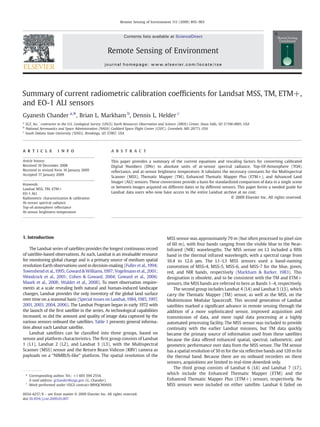
  • 6. Tables 2–5 give the prelaunch “measured” (as-built performance) spectral ranges. These numbers are slightly different from the original filter specification. The center wavelengths are the average of the two spectral range numbers. Figs.1 and 2 show the Relative Spectral Response (RSR) profiles of the Landsat MSS (Markham Barker, 1983), TM (Markham Barker, 1985), ETM+(Handbook2 ), and ALI (Mendenhall Parker, 1999) sensors measured during prelaunch characterization. The ETM+ spectral bands were designed to mimic the standard TM spectral bands 1–7. The ALI bands were designed to mimic the six standard ETM+ solar reflective spectral bands 1–5, and 7; three new bands,1p, 4p, and 5p, were added to more effectively address atmospheric interference effects and specific applications. The ALI band numbering corresponds with the ETM+ spectral bands. Bands not present on the ETM+ sensor are given the “p,” or prime, designation. MSS spectral bands are significantly different from TM and ETM+ spectral bands. The post-calibration dynamic ranges are band-specific rescaling factors typically provided in the Level 1 product header file. Over the life of the Landsat sensors, occasional changes have occurred in Fig. 1. Comparison of the solar reflective bands RSR profiles of L1–5 MSS sensors. 898 G. Chander et al. / Remote Sensing of Environment 113 (2009) 893–903
  • 7. the post-calibration dynamic range. Future changes are anticipated, especially in the MSS and TM data, because of the possible adjustment of the calibration constants based on comparisons to absolute radiometric measurements made on the ground. In some cases, the header file may have different rescaling factors than provided in the table included here. In these cases, the user should use the header file information that comes with the product. Two processing systems will continue to generate Landsat data products: the Level 1 Product Generation System (LPGS) and the National Land Archive Production System (NLAPS). Starting December 8, 2008, all L7 ETM+ and L5 TM (except Thematic Mapper-Archive [TM-A]8 products) standard Level 1 products are processed through the LPGS, and all L4 TM and MSS standard Level 1 products are processed through the NLAPS. The Landsat Program is working toward transitioning the processing of all Landsat data to LPGS (Kline, personal 8 A small number of TM scenes were archived as radiometrically corrected products known as TM-A data. The TM-A data are archived on a scene-by-scene basis (instead of intervals). The L4 and L5 TM-A scenes will continue to be processed using NLAPS (with Qcalmin =0), which attempts to uncalibrate the previously applied calibration and generates the product using updated calibration procedures. Note that approximately 80 L4 TM and approximately 13,300 L5 TM scenes are archived as TM-A data, with acquisition dates ranging between Sept.1982 and Aug. 1990. Fig. 2. Comparison of the solar reflective bands RSR profiles of L4 TM, L5 TM, L7 ETM+, and EO-1 ALI sensors. 899G. Chander et al. / Remote Sensing of Environment 113 (2009) 893–903
  • 8. communication). In mid-2009, the processing of L4 TM data will transition from NLAPS to LPGS. The scenes processed using LPGS include a header file (.MTL), which lists the LMINλ and LMAXλ values but not the rescaling gain and bias numbers. The scenes processed using NLAPS include a processing history work order report (.WO), which lists the rescaling gain and bias numbers but not the LMINλ and LMAXλ. The sensitivity of the detector changes over time, causing a change in the detector gain applied during radiometric calibration. However, the numbers presented in Tables 2–5 are the rescaling factors, which are the post-calibration dynamic ranges. The LMINλ and LMAXλ are a repre- sentation of how the output Landsat Level 1 data products are scaled in at-sensor radiance units. Generally, there is no need to change the LMINλ or LMAXλ unless something changes drastically on the sensor. Thus, there is notime dependence for any of the rescaling factors inTables 2–5. 5. Conversion to TOA reflectance (Lλ-to-ρP) A reduction in scene-to-scene variability can be achieved by converting the at-sensor spectral radiance to exoatmospheric TOA reflectance, also known as in-band planetary albedo. When comparing images from different sensors, there are three advantages to using TOA reflectance instead of at-sensor spectral radiance. First, it removes the cosine effect of different solar zenith angles due to the time difference between data acquisitions. Second, TOA reflectance compensates for different values of the exoatmospheric solar irradiance arising from spectral band differences. Third, the TOA reflectance corrects for the variation in the Earth–Sun distance between different data acquisition dates. These variations can be significant geographically and temporally. The TOA reflectance of the Earth is computed according to the equation: ρλ = π Á Lλ Á d2 ESUNλ Á cos θs ð2Þ where ρλ= Planetary TOA reflectance [unitless] π= Mathematical constant equal to ~3.14159 [unitless] Lλ= Spectral radiance at the sensor's aperture [W/(m2 sr μm)] d= Earth–Sun distance [astronomical units] ESUNλ= Mean exoatmospheric solar irradiance [W/(m2 μm)] θs= Solar zenith angle [degrees9 ] Note that the cosine of the solar zenith angle is equal to the sine of the solar elevation angle. The solar elevation angle at the Landsat scene center is typically stored in the Level 1 product header file (.MTL or .WO) or retrieved from the USGS EarthExplorer or GloVis online interfaces under the respective scene metadata (these web sites also contain the acquisition time in hours, minutes, and seconds). The TOA reflectance calculation requires the Earth–Sun distance (d). Table 6 presents d in astronomical units throughout a year generated using the Jet Propulsion Laboratory (JPL) Ephemeris10 (DE405) data. The d numbers are also tabulated in the Nautical Almanac Office. The last column of Tables 2–5 summarizes solar exoatmospheric spectral irradiances (ESUNλ) for the MSS, TM, ETM+, and ALI sensors using the Thuillier solar spectrum (Thuillier et al., 2003). The Committee on Earth Observation Satellites (CEOS) Working Group on Calibration and Validation (WGCV) recommends11 using this spectrum for applications in optical-based Earth Observation that use an exoatmospheric solar irradiance spectrum. The Thuillier spectrum is believed to be the most accurate and an improvement over the other solar spectrum. Note that the CHKUR solar spectrum in MODTRAN 4.0 (Air Force Laboratory,1998) was used previously for ETM+(Handbook2 ) and TM (Chander Markham, 2003), whereas the Neckel and Lab (Neckel Labs,1984) and Iqbal (Iqbal, 1983) solar spectrums were used for MSS and TM solar irradiance values (MarkhamBarker,1986).Theprimarydifferences occurin Bands5 and7. For comparisons to other sensors, users need to verify that the same solar spectrum is used for all sensors. 6. Conversion to at-sensor brightness temperature (Lλ-to-T) The thermal band data (Band 6 onTM and ETM+) can be converted from at-sensor spectral radiance to effective at-sensor brightness temperature. The at-sensor brightness temperature assumes that the Earth's surface is a black body (i.e., spectral emissivity is 1), and includes atmospheric effects (absorption and emissions along path). The at-sensor temperature uses the prelaunch calibration constants given in Table 7. The conversion formula from the at-sensor's spectral radiance to at-sensor brightness temperature is: T = K2 ln K1 Lλ + 1 ð3Þ where: T= Effective at-sensor brightness temperature [K] K2= Calibration constant 2 [K] Fig. 2 (continued). 9 Note that Excel, Matlab, C, and many other software applications use radians, not degrees, to perform calculations. The conversion from degrees to radians is a multiplication factor of pi/180. 10 http://ssd.jpl.nasa.gov/?horizons. 11 CEOS-recommended solar irradiance spectrum, http://wgcv.ceos.org. 900 G. Chander et al. / Remote Sensing of Environment 113 (2009) 893–903
  • 9. K1= Calibration constant 1 [W/(m2 sr μm)] Lλ= Spectral radiance at the sensor's aperture [W/(m2 sr μm)] ln= Natural logarithm The ETM+ Level 1 product has two thermal bands, one acquired using a low gain setting (often referred to as Band 6 L; useful temperature range of 130–350 K) and the other using a high gain setting (often referred to as Band 6H; useful temperature range of 240–320 K). The noise equivalent change in temperature (NEΔT) at 280 K for ETM+ high gain is 0.22 and for low gain is 0.28. The TM Level 1 product has only one thermal band (there is no gain setting on the TM sensor), and the thermal band images have a useful temperature Table 6 Earth–Sun distance (d) in astronomical units for Day of the Year (DOY). DOY d DOY d DOY d DOY d DOY d DOY d 1 0.98331 61 0.99108 121 1.00756 181 1.01665 241 1.00992 301 0.99359 2 0.98330 62 0.99133 122 1.00781 182 1.01667 242 1.00969 302 0.99332 3 0.98330 63 0.99158 123 1.00806 183 1.01668 243 1.00946 303 0.99306 4 0.98330 64 0.99183 124 1.00831 184 1.01670 244 1.00922 304 0.99279 5 0.98330 65 0.99208 125 1.00856 185 1.01670 245 1.00898 305 0.99253 6 0.98332 66 0.99234 126 1.00880 186 1.01670 246 1.00874 306 0.99228 7 0.98333 67 0.99260 127 1.00904 187 1.01670 247 1.00850 307 0.99202 8 0.98335 68 0.99286 128 1.00928 188 1.01669 248 1.00825 308 0.99177 9 0.98338 69 0.99312 129 1.00952 189 1.01668 249 1.00800 309 0.99152 10 0.98341 70 0.99339 130 1.00975 190 1.01666 250 1.00775 310 0.99127 11 0.98345 71 0.99365 131 1.00998 191 1.01664 251 1.00750 311 0.99102 12 0.98349 72 0.99392 132 1.01020 192 1.01661 252 1.00724 312 0.99078 13 0.98354 73 0.99419 133 1.01043 193 1.01658 253 1.00698 313 0.99054 14 0.98359 74 0.99446 134 1.01065 194 1.01655 254 1.00672 314 0.99030 15 0.98365 75 0.99474 135 1.01087 195 1.01650 255 1.00646 315 0.99007 16 0.98371 76 0.99501 136 1.01108 196 1.01646 256 1.00620 316 0.98983 17 0.98378 77 0.99529 137 1.01129 197 1.01641 257 1.00593 317 0.98961 18 0.98385 78 0.99556 138 1.01150 198 1.01635 258 1.00566 318 0.98938 19 0.98393 79 0.99584 139 1.01170 199 1.01629 259 1.00539 319 0.98916 20 0.98401 80 0.99612 140 1.01191 200 1.01623 260 1.00512 320 0.98894 21 0.98410 81 0.99640 141 1.01210 201 1.01616 261 1.00485 321 0.98872 22 0.98419 82 0.99669 142 1.01230 202 1.01609 262 1.00457 322 0.98851 23 0.98428 83 0.99697 143 1.01249 203 1.01601 263 1.00430 323 0.98830 24 0.98439 84 0.99725 144 1.01267 204 1.01592 264 1.00402 324 0.98809 25 0.98449 85 0.99754 145 1.01286 205 1.01584 265 1.00374 325 0.98789 26 0.98460 86 0.99782 146 1.01304 206 1.01575 266 1.00346 326 0.98769 27 0.98472 87 0.99811 147 1.01321 207 1.01565 267 1.00318 327 0.98750 28 0.98484 88 0.99840 148 1.01338 208 1.01555 268 1.00290 328 0.98731 29 0.98496 89 0.99868 149 1.01355 209 1.01544 269 1.00262 329 0.98712 30 0.98509 90 0.99897 150 1.01371 210 1.01533 270 1.00234 330 0.98694 31 0.98523 91 0.99926 151 1.01387 211 1.01522 271 1.00205 331 0.98676 32 0.98536 92 0.99954 152 1.01403 212 1.01510 272 1.00177 332 0.98658 33 0.98551 93 0.99983 153 1.01418 213 1.01497 273 1.00148 333 0.98641 34 0.98565 94 1.00012 154 1.01433 214 1.01485 274 1.00119 334 0.98624 35 0.98580 95 1.00041 155 1.01447 215 1.01471 275 1.00091 335 0.98608 36 0.98596 96 1.00069 156 1.01461 216 1.01458 276 1.00062 336 0.98592 37 0.98612 97 1.00098 157 1.01475 217 1.01444 277 1.00033 337 0.98577 38 0.98628 98 1.00127 158 1.01488 218 1.01429 278 1.00005 338 0.98562 39 0.98645 99 1.00155 159 1.01500 219 1.01414 279 0.99976 339 0.98547 40 0.98662 100 1.00184 160 1.01513 220 1.01399 280 0.99947 340 0.98533 41 0.98680 101 1.00212 161 1.01524 221 1.01383 281 0.99918 341 0.98519 42 0.98698 102 1.00240 162 1.01536 222 1.01367 282 0.99890 342 0.98506 43 0.98717 103 1.00269 163 1.01547 223 1.01351 283 0.99861 343 0.98493 44 0.98735 104 1.00297 164 1.01557 224 1.01334 284 0.99832 344 0.98481 45 0.98755 105 1.00325 165 1.01567 225 1.01317 285 0.99804 345 0.98469 46 0.98774 106 1.00353 166 1.01577 226 1.01299 286 0.99775 346 0.98457 47 0.98794 107 1.00381 167 1.01586 227 1.01281 287 0.99747 347 0.98446 48 0.98814 108 1.00409 168 1.01595 228 1.01263 288 0.99718 348 0.98436 49 0.98835 109 1.00437 169 1.01603 229 1.01244 289 0.99690 349 0.98426 50 0.98856 110 1.00464 170 1.01610 230 1.01225 290 0.99662 350 0.98416 51 0.98877 111 1.00492 171 1.01618 231 1.01205 291 0.99634 351 0.98407 52 0.98899 112 1.00519 172 1.01625 232 1.01186 292 0.99605 352 0.98399 53 0.98921 113 1.00546 173 1.01631 233 1.01165 293 0.99577 353 0.98391 54 0.98944 114 1.00573 174 1.01637 234 1.01145 294 0.99550 354 0.98383 55 0.98966 115 1.00600 175 1.01642 235 1.01124 295 0.99522 355 0.98376 56 0.98989 116 1.00626 176 1.01647 236 1.01103 296 0.99494 356 0.98370 57 0.99012 117 1.00653 177 1.01652 237 1.01081 297 0.99467 357 0.98363 58 0.99036 118 1.00679 178 1.01656 238 1.01060 298 0.99440 358 0.98358 59 0.99060 119 1.00705 179 1.01659 239 1.01037 299 0.99412 359 0.98353 60 0.99084 120 1.00731 180 1.01662 240 1.01015 300 0.99385 360 0.98348 361 0.98344 362 0.98340 363 0.98337 364 0.98335 365 0.98333 366 0.98331 901G. Chander et al. / Remote Sensing of Environment 113 (2009) 893–903
  • 10. range of 200–340 K. The NEΔT at 280 K for L5 TM is 0.17–0.30 (Barsi et al., 2003). 7. Conclusion This paper provides equations and rescaling factors for converting Landsat calibrated DNs to absolute units of at-sensor spectral radiance, TOA reflectance, and at-sensor brightness temperature. It tabulates the necessary constants for the MSS, TM, ETM+, and ALI sensors in a coherent manner using the same units and definitions. This paper forms a needed guide for Landsat data users who now have access to the entire Landsat archive at no cost. Studies are ongoing to evaluate the MSS calibration consistency and provide post-calibration adjustments of the MSS sensors so they are consistent over time and consistent between sensors. Further updates to improve the TM and ETM+ thermal band calibration are being investigated, as is the calibration of the L4 TM. Acknowledgments This work was partially supported by the NASA Land-Cover and Land-Use Change (LCLUC) Grant NNH08AI30I. The authors acknowl- edge the support of David Aaron (SDSU) for digitizing the spectral responses for the MSS sensors and Julia Barsi (SSAI) for generating the Earth–Sun distance. Special thanks are extended to a number of colleagues for reviewing drafts of this manuscript. The anonymous reviewers' comments were particularly valuable and their efforts are greatly appreciated. Any use of trade, product, or firm names is for descriptive purposes only and does not imply endorsement by the U.S. Government. Appendix A References Air Force Research Laboratory (1998). Modtran Users Manual, Versions 3.7 and 4.0 : Hanscom Air Force Base, MA. Barsi, J. A., Schott, J. R., Palluconi, F. D., Helder, D. L., Hook, S. J., Markham, B. L., Chander, G., O'Donnell, E. M. (2003). Landsat TM and ETM+ thermal band calibration. Canadian Journal of Remote Sensing, 29(2), 141−153. Barsi, J. A., Hook, S. J., Schott, J. R., Raqueno, N. G., Markham, B. L. (2007). Landsat-5 Thematic Mapper thermal band calibration update. IEEE Transactions on Geoscience and Remote Sensing, 44, 552−555. Chander, G., Markham, B. L. (2003). Revised Landsat-5 TM radiometric calibration procedures, and post-calibration dynamic ranges. IEEE Transactions on Geoscience and Remote Sensing, 41, 2674−2677. Chander, G., Helder, D. L., Markham, B. L., Dewald, J., Kaita, E., Thome, K. J., Micijevic, E., Ruggles, T. (2004a). Landsat 5 TM on-orbit absolute radiometric performance. IEEE Transactions on Geoscience and Remote Sensing, 42, 2747−2760. Chander, G., Meyer, D. J., Helder, D. L. (2004b). Cross-calibration of the Landsat-7 ETM+ and EO-1 ALI sensors. IEEE Transactions on Geoscience and Remote Sensing, 42(12), 2821−2831. Chander, G., Markham, B. L., Barsi, J. A. (2007a). Revised Landsat 5 Thematic Mapper radiometric calibration.IEEE Transactions on Geoscience and Remote Sensing,44, 490−494. Chander, G., Angal, A., Choi, T., Meyer, D. J., Xiong, X., Teillet, P. M. (2007b). Cross- calibration of the Terra MODIS, Landsat-7 ETM+ and EO-1 ALI sensors using near simultaneous surface observation over Railroad Valley Playa, Nevada test site. In J. J. Butler J. Xiong (Eds.), Proceedings of SPIE Conference 6677 on Earth Observing Systems XII, SPIE, Vol. 6677. (pp. 66770Y: 1−12) San Diego, CA. Chander, G., Coan, M. J., Scaramuzza, P. L. (2008). Evaluation and comparison of the IRS-P6 and the Landsat Sensors. IEEE Transactions on Geoscience and Remote Sensing, 46(1), 209−221. Cohen, W. B., Goward, S. N. (2004). Landsat's role in ecological applications of remote sensing. BioScience, 54(6), 535−545. Fuller, R. M., Groom, G. B., Jones, A. R. (1994). The land cover map of Great Britain: An automated classification of Landsat Thematic Mapper data. Photogrammetric Engineering and Remote Sensing, 60, 553−562. Goward, S. N., Williams, D. L. (1997). Landsat and Earth Systems Science: Development of terrestrial monitoring.Photogrammetric Engineering and Remote Sensing,63(7), 887−900. Goward, S., Irons, J., Franks, S., Arvidson, T., Williams, D., Faundeen, J. (2006). Historical record of Landsat global coverage: Mission operations, NSLRSDA, and international cooperator stations. Photogrammetric Engineering and Remote Sensing, 72, 1155−1169. GSFC Specification for the Thematic Mapper System and Associated Test Equipment. (Rev C., January 1981) GSFC 400-8-D-210C, NASA, Goddard Space Flight Center, Greenbelt, MD. Helder, D. L. (1993). MSS radiometric calibration handbook. Report to the U.S. Geological Survey (USGS) Earth Resources Observation and Science (EROS) Center. Helder, D. L., Boncyk, W. C., Morfitt, R. (1998). Absolute calibration of the Landsat Thematic Mapper using the internal calibrator. Proc. IGARSS, Seattle, WA, 1998 (pp. 2716−2718). Helder, D. L. (2008a). Consistent radiometric calibration of the historical Landsat archive. Proceedings of PECORA Denver, Colorado. Helder, D. L., Markham, B. L., Thome, K. J., Barsi, J. A., Chander, G., Malla, R. (2008b). Updated radiometric calibration for the Landsat 5 Thematic Mapper reflective bands. IEEE Transactions on Geoscience and Remote Sensing, 46(10), 3309−3325. Helder, D.L., Ruggles, T. A. (2004a). Landsat ThematicMapper reflectiveband radiometric artifacts. IEEE Transactions on Geoscience and Remote Sensing, 44, 2704−2716. Helder, D. L., Ruggles, T. A., Dewald, J. D., Madhavan, S. (2004b). Landsat-5 Thematic Mapper reflective-band radiometric stability. IEEE Transactions on Geoscience and Remote Sensing, 44, 2704−2716. Iqbal, M. (1983). Introduction to solar radiation. New York: Academic Press. Markham, B. L., Barker, J. L. (1983). Spectral characterization of the Landsat-4 MSS sensors. Photogrammetric Engineering and Remote Sensing, 49(6), 811−833. Markham, B. L., Barker, J. L. (1985). Spectral characterization of the LANDSAT Thematic Mapper sensors'. International Journal of Remote Sensing, 6(5), 697−716. Markham, B. L., Barker, J. L. (1986). Landsat MSS and TM post-calibration dynamic ranges, exoatmospheric reflectances and at-satellite temperatures. Earth Observa- tion Satellite Co., Lanham, MD, Landsat Tech. Note 1. Markham, B. L., Barker, J. L. (1987). Radiometric properties of U.S. processed Landsat MSS Data. Remote Sensing of Environment, 22, 39−71. Markham, B. L., Seiferth, J. C., Smid, J., Barker, J. L. (1998). Lifetime responsivity behavior of the Landsat-5 Thematic Mapper. Proceedings of SPIE Conference 3427 on Earth Observing Systems, SPIE, Vol. 3427. (pp. 420−431) San Diego, CA. Markham, B. L., Chander, G., Morfitt, R., Hollaren, D., Mendenhall, J. F., Ong, L. (2004a). Radiometric processing and calibration of EO-1 Advanced Land Imager data. Proceedings of PECORA 16 “Global Priorities in Land Remote Sensing” South Dakota: Sioux Falls. Table A1 To maintain consistency, all Landsat scenes are based on the following naming convention. Format Example: LXSPPPRRRYYYYDDDGSIVV L=Landsat Sensor Examples: LM10170391976031AAA01(MSS) LT40170361982320XXX08 (TM) LE70160392004262EDC02 (ETM+)X=Sensor S=Satellite PPP = Worldwide Reference System (WRS) Path RRR=WRS Row YYYY=Year DDD=Day of Year GSI=Ground Station Identifier ⁎ VV=Version ⁎Ground Stations Identifiers-Data received at these sites are held at EROS AAA=North American site unknown GNC=Gatineau, Canada ASA=Alice Springs, Australia LGS=EROS, SD, USA, Landsat 5 data acquired by EROS beginning July 1, 2001FUI=Fucino, Italy (Historical) GLC=Gilmore Creek, AK, US MOR=Moscow, Russia HOA=Hobart, Australia MLK=Malinda, Kenya KIS=Kiruna, Sweden IKR=Irkutsk, Russia MTI=Matera, Italy CHM=Chetumal, Mexico EDC=Receiving site unknown XXO=Receiving site unknown PAC=Prince Albert, Canada XXX=Receiving site unknown Table A2 Standard Level 1 product specifications. Product Type – Level 1T (Terrain Corrected) Pixel Size – 15/30/60 meters Output format – GeoTIFF Resampling Method – Cubic Convolution (CC) Map Projection – Universal Transverse Mercator (UTM) Polar Stereographic for Antarctica Image Orientation – Map (North Up) Distribution – File Transfer Protocol (FTP) Download only Table 7 TM and ETM+ thermal band calibration constants. Constant K1 K2 Units W/(m2 sr μm) Kelvin L4 TM 671.62 1284.30 L5 TM 607.76 1260.56 L7 ETM+ 666.09 1282.71 902 G. Chander et al. / Remote Sensing of Environment 113 (2009) 893–903
  • 11. Markham, B. L., Thome, K., Barsi, J., Kaita, E., Helder, D., Barker, J., Scaramuzza, P. (2004b). Landsat-7 ETM+ On-Orbit reflective-band radiometric stability and absolute calibra- tion. IEEE Transactions on Geoscience and Remote Sensing, 42, 2810−2820. Markham, B. L., Ong, L., Barsi, J. A., Mendenhall, J. A., Lencioni, D. E., Helder, D. L., Hollaren, D. H., Morfitt, R. M. (2006). Radiometric calibration stability of the EO-1 Advanced Land Imager: 5 Years on-orbit. In R. Meynart, S. P. Neeck, H. Shimoda (Eds.), Proceedings of SPIE Conference 6361 on Sensors, Systems, and Next-Generation Satellites X, SPIE, Vol. 6361. (pp. 66770U: 1−12) San Diego, CA. Masek, J. G., Vermote, Huang, C., Wolfe, R., Cohen, W., Hall, F., Kutler, J., Nelson, P. (2008). North American forest disturbance mapped from a decadal Landsat record. Remote Sensing of Environment, 112, 2914−2926. Mendenhall, J. A., Parker, A. C. (1999). Spectral calibration of the EO-1 Advanced Land Imager. Proceedings of SPIE Conference 3750 on Earth Observing Systems IV, SPIE, Vol. 3750. (pp. 109−116) Denver, Colorado. Mendenhall, J. A., Lencioni, D.E. (2002). EO-1 advanced land imageron-orbit radiometric calibration. International Geoscience and Remote Sensing Symposium Toronto, Canada. Nautical Almanac Office. The Nautical Almanac for the Year (United States Naval Observatory) (Washington, DC: U.S. Government Printing Office). Neckel, H., Labs, D. (1984). The solar radiation between 3300 and 12500 A. Solar Physics, 90, 205. Roy, D., Borak, J., Devadiga, S., Wolfe, R., Zheng, M., Descloitres, J. (2002). The MODIS land product quality assessment approach. Remote Sensing of Environment, 83, 62−76. Special Issue on Landsat 4 (1984). IEEE Transactions on Geoscience and Remote Sensing, GE-22(3), 160 51(9). Guest Editor: Solomonson, V.V. Special Issue on Landsat Image Data Quality Analysis (LIDQA) (1985). Photogrammetric Engineering and Remote Sensing, 51(9) Guest Editors: Markham, B.L., and Barker, J.L. Special Issue on 25th Anniversary of Landsat (1997). Photogrammetric Engineering and Remote Sensing, 63(7) Guest Editor: Salomonson, V.V. Special Issue on Landsat 7 (2001). Remote Sensing of Environment, 78(1–2), 1−220 Guest Editors: Goward, S.N., and Masek, J.G. Special Issue on Synergistic Utilization of Landsat 7 (2003). Canadian Journal of Remote Sensing, 29(2), 141−297 Guest Editor: Teillet, P.M. Special Issue on Landsat Sensor Performance Characterization (2004). IEEE Transactions on Geoscience and Remote Sensing, 42(12), 2687−2855 Guest Editors: Markham, B.L., Storey, J.C., Crawford, M.M., Goodenough, D.G., Irons, J.R. Special Issue on Landsat Operations: Past, Present and Future (2006). Photogrammetric Engineering and Remote Sensing, 72(10) Guest Editors: Williams, D.L, Goward, S.N., Arvidson, T. Storey, J. C., Scaramuzza, P., Schmidt, G. (2005). Landsat 7 scan line corrector-off gap filled product development. PECORA 16 Conference Proceedings, Sioux Falls, South Dakota (pp. 23−27). Teillet, P. M., Barker, J. L., Markham, B. L., Irish, R. R., Fedosejeves, G., Storey, J. C. (2001). Radiometric cross-calibration of the Landsat-7 ETM+ and Landsat-5 TM sensors based on tandem data sets. Remote Sensing of Environment, 78(1–2), 39−54. Teillet, P. M., Helder, D. L., Ruggles, T. A., Landry, R., Ahern, F. J., Higgs, N. J., et al. (2004). A definitive calibration record for the Landsat-5 Thematic Mapper anchored to the Landsat-7 radiometric scale. Canadian Journal of Remote Sensing, 30(4), 631−643. Teillet, P. M., Markham, B. L., Irish, R. R. (2006). Landsat cross-calibration based on near simultaneous imaging of common ground targets. Remote Sensing of Environment, 102 (3–4), 264−270. Teillet, P. M., Fedosejevs, G., Thome, K. J., Barker, J. L. (2007). Impacts of spectral band difference effects on radiometric cross-calibration between satellite sensors in the solar-reflective spectral domain. Remote Sensing of Environment, 110, 393−409. Thome, K. J. (2001). Absolute radiometric calibration of Landsat 7 ETM+ using the reflectance-based method. Remote Sensing of Environment, 78(1–2), 27−38. Thome, K. J., Markham, B. L., Barker, J. L., Slater, P. L., Biggar, S. (1997a). Radiometric calibration of Landsat. Photogrammetric Engineering and Remote Sensing, 63, 853−858. Thome, K. J., Crowther, B. G., Biggar, S. F. (1997b). Reflectance- and irradiance-based calibration of Landsat-5 Thematic Mapper. Canadian Journal of Remote Sensing, 23, 309−317. Thome, K. J., Biggar, S. F., Wisniewski, W. (2003). Cross comparison of EO-1 sensors and other earth resources sensors to Landsat-7 ETM+ using Railroad Valley Playa. IEEE Transactions on Geoscience and Remote Sensing, 41, 1180−1188. Thome, K. J., Helder, D. L., Aaron, D. A., Dewald, J. (2004). Landsat 5 TM and Landsat-7 ETM+ absolute radiometric calibration using reflectance based method. IEEE Transactions on Geoscience and Remote Sensing, 42(12), 2777−2785. Thuillier, G., Herse, M., Labs, S., Foujols, T., Peetermans, W., Gillotay, D., Simon, P. C., Mandel, H. (2003). The solar spectral irradiance from 200 to 2400 nm as measured by SOLSPEC Spectrometer from the ATLAS 123 and EURECA missions.Solar Physics, 214(1), 1−22 Solar Physics. Townshend, J. R. G., Bell, V., Desch, A. C., Havlicek, C., Justice, C. O., Lawrence, W. E., Skole, D., Chomentowski, W. W., Moore, B., Salas, W., Tucjer, C. J. (1995). The NASA Landsat Pathfinder Humid Tropical Deforestation Project. Proceedings Land Satellite Information in the Next Decade, ASPRS Conference (pp. 76−87). Vienna, Virginia. Vogelmann, J. E., Howard, S. M., Yang, L., Larson, C. R., Wylie, B. K., Van Driel, J. N. (2001). Completion of the 1990's National Land Cover Data Set for the conterminous United States. Photogrammetric Engineering and Remote Sensing, 67, 650−662. Woodcock, C. E., Macomber, S. A., Pax-Lenney, M., Cohen, W. C. (2001). Monitoring large areas for forest change using Landsat: Generalization across space, time and Landsat sensors. Remote Sensing of Environment, 78, 194−203. Woodcock, C. E., Allen, A. A., Anderson, M., Belward, A. S., Bindschadler, R., Cohen, W. B., Gao, F., Goward, S. N., Helder, D., Helmer, E., Nemani, R., Oreapoulos, L., Schott, J., Thenkabail, P. S., Vermote, E. F., Vogelmann, J., Wulder, M. A., Wynne, R. (2008). Free access to Landsat imagery. Science, 320, 1011. Wulder, M. A., White, J. C., Goward, S. N., Masek, J. G., Irons, J. R., Herold, M., Cohen, W. B., Loveland, T. R., Woodcock, C. E. (2008). Landsat continuity: Issues and opportunities for land cover monitoring. Remote Sensing of Environment, 112, 955−969. 903G. Chander et al. / Remote Sensing of Environment 113 (2009) 893–903