2. 50 2 Diagrams
Let Γ be a geometry over I . The digon diagram I(Γ ) of Γ is the graph whose
vertex set is I and whose edges are the pairs {i, j } from I for which there is a residue
of type {i, j } that is not a generalized digon.
In other words, a generalized digon has a complete bipartite incidence graph.
The choice of the name digon will become clear in Sect. 2.2, where the notion of
generalized polygon is introduced.
Example 2.1.2 In the examples of Sect. 1.1, the cube, the icosahedron, a polyhe-
dron, a tessellation of E2 , and the Euclidean space E3 all have digon diagram
◦ ◦ ◦.
The digon diagram of Example 1.1.5 (tessellation of E3 by polyhedra) is
◦ ◦ ◦ ◦.
The digon diagram of a geometry Γ is a concise way of capturing some of the
structure of Γ . This information is called local as it involves rank two residues only.
The usefulness of the digon diagram can be illustrated as follows. Assume that
we are looking for all auto-correlations of Γ . It is obvious that each auto-correlation
α of Γ permutes the types of Γ , inducing a permutation on I that is an automor-
phism of I(Γ ). If I(Γ ) is linear, that is, has the shape of single path, we see at
once that I(Γ ) has exactly two automorphisms: the identity and an involution per-
muting the endpoints of I(Γ ). This implies that Γ has at most two families of auto-
correlations: automorphisms and dualities (interchanging elements whose types are
at the extreme ends of I(Γ ), such as points and hyperplanes in projective geome-
tries). The latter need not exist, as can be seen from the cube geometry of rank three;
its dual geometry is the octahedron, which is not isomorphic to the original cube.
The digon diagram of a geometry is not necessarily linear. The digon diagram of
Example 1.3.10, for instance, is a triangle. Actually every graph is the digon diagram
of some geometry. Nevertheless, most of the geometries studied in this book have
a digon diagram that is close to being linear. We now give some examples with
non-linear digon diagrams.
Example 2.1.3 Consider the geometry constructed from a tessellation of E3 by
cubes discussed in Example 1.1.5. Up to Euclidean isometry, there is a unique way
to color the vertices with two colors b (for black) and w (for white), and the cubes
(the cells) with two other colors g (for green) and r (for red) in such a way that
two adjacent vertices (respectively, cubes) do not bear the same color. Let Γ be the
geometry over {b, w, g, r} on the bicolored vertices and cubes; incidence is sym-
metrized inclusion for vertices and cubes, and adjacency for two vertices, as well as
for two cubes. The digon diagram of Γ is a quadrangle in which b and w represent
opposite vertices and g and r likewise. Here, and elsewhere, a quadrangle is a cir-
cuit of length four without further adjacencies; in other words a complete bipartite
graph with two parts of size two each.
3. 2.1 The Digon Diagram of a Geometry 51
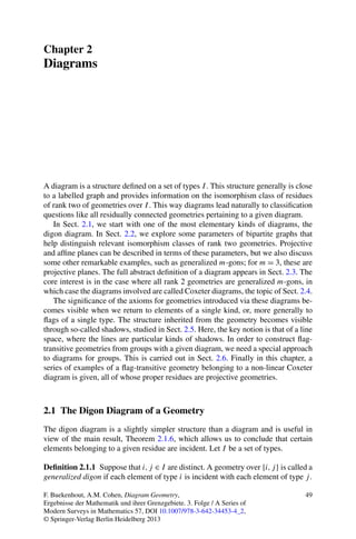
Fig. 2.1 The digon diagram
of Δ from Example 2.1.3
For a variation, consider the geometry Δ over {v, e, g, r} whose elements of
type g and r are as above, and whose elements of type v and e are the vertices and
edges of the tessellation, respectively. Define incidence by the Principle of Maxi-
mal Intersection (cf. Exercise 1.9.20). Then the digon diagram of Δ is as indicated
in Fig. 2.1.
There is a relation between the digon diagram of Γ and those of its residues. We
will use the notion partial subgraph introduced in Definition 1.2.1.
Proposition 2.1.4 Let Γ be a geometry over I and let F be a flag of Γ . The digon
diagram I(ΓF ) is a partial subgraph of the digon diagram I(Γ ).
Proof It suffices to apply Proposition 1.5.3 and to see that every residue of type
{i, j } in ΓF is also a residue of type {i, j } in Γ .
Remark 2.1.5 It may happen that two vertices of I(ΓF ) are not joined while they
are joined in I(Γ ). Of course, the digon diagram I(ΓF ) is a subgraph of I(Γ ) for
all flags F if and only if, for any two distinct types i, j , either all or none of the
residues in Γ of type {i, j } are generalized digons. This property holds for flag-
transitive geometries and for most of the geometries we study later. It gives rise to a
useful heuristic trick. Given such a ‘pure’ geometry Γ , its digon diagram I(Γ ), and
a flag F , it suffices to remove the vertices of τ (F ) from I(Γ ) as well as the edges
having a vertex in τ (F ) in order to obtain the digon diagram of ΓF .
Theorem 2.1.6 (Direct Sum) Let Γ be a residually connected geometry of finite
rank and let i and j be types in distinct connected components of the digon diagram
I(Γ ). Then every element of type i in Γ is incident with every element of type j
in Γ .
Proof Write Γ = (X, ∗, τ ) and r = rk(Γ ). We proceed by induction on r. For r = 2,
the graph I(Γ ) consists of the non-adjacent vertices i and j , so Γ is a generalized
digon, for which the theorem obviously holds. Let r ≥ 3, and let k be an element
of I = τ (X) distinct from i, j . As i and j are in distinct connected components
of I(Γ ), we may assume that k and i are not in the same connected component
of I(Γ ). Let xi (respectively, xj ) be an element of type i (respectively, j ). By
Lemma 1.6.3, there is an {i, j }-chain from xi to xj in Γ . We must show that xi , xj
is such a path.
4. 52 2 Diagrams
Suppose that we have xi ∗ yj ∗ yi ∗ xj with yj ∈ Xj , yi ∈ Xi . By Corol-
lary 1.6.6 applied to the flag {yi }, there is a {j, k}-chain from yj to xj in Γyi , say
yj = yj , zk , yj , zk , . . . , zk , xj , with zk ∈ Xk and yj ∈ Xj for all m ∈ [s]. By Propo-
1 1 2 2 s m m
sition 2.1.4, the types i and k are in distinct connected components of I(Γyj ) and
by the induction hypothesis we obtain xi ∗ zk . Similarly, in Γz1 , we find xi ∗ yj .
1 2
k
Repeated use of this argument eventually leads to xi ∗ xj .
The preceding paragraph shows that an {i, j }-chain of length m ≥ 3 between an
element of Xi and an element of Xj can be shortened to an {i, j }-chain between the
same endpoints of length m − 2. Hence the minimal length of such a path, being
odd, must be 1.
In view of Exercise 2.8.20, the condition that I has finite cardinality is needed in
Theorem 2.1.6.
Remark 2.1.7 Interesting geometries tend to have a connected digon diagram. How-
ever such a geometry may have residues whose digon diagrams are no longer con-
nected. Take for instance a residually connected geometry Γ over [3] whose digon
diagram is
1 2 3 4
◦ ◦ ◦ ◦.
If x is an element of type 2, then any element of type 1 and any element of type 3,
both incident with x, are necessarily incident with each other. This is the kind of use
we will make of the Direct Sum Theorem 2.1.6.
A consequence of the theorem is that any residually connected geometry of finite
rank with a disconnected digon diagram can be seen as a direct sum of geometries
whose digon diagrams are connected.
Definition 2.1.8 Let J be a set of indices and (Ij )j ∈J a system of pairwise disjoint
sets. Let Γj = (Xj , ∗j , τj ) be a geometry over Ij where (Xj )j ∈J is a system of
pairwise disjoint sets. The direct sum of the geometries Γj (j ∈ J ) is the triple
Γ = (X, ∗, τ ) where X = j ∈J Xj , ∗|Xj = ∗j , x ∗ y for x ∈ Xj , y ∈ Xk , j = k,
and τ |Xj = τj .
Example 2.1.9 A direct sum of two rank one geometries is a generalized digon. Any
generalized digon is obtained in this way.
For the direct sum Γ as in Definition 2.1.8, it is clear that Γ is a geometry over
I = j ∈J Ij whose digon diagram I(Γ ) is the disjoint union of the digon diagrams
I(Γj ) for j ∈ J . Here is a converse of this statement.
Corollary 2.1.10 Let Γ be a residually connected geometry of finite rank. Let
(Ij )j ∈J be the collection of all connected components of the digon diagram I(Γ ).
Then Γ is isomorphic to the direct sum of the Ij -truncations Ij Γ (j ∈ J ) of Γ .
5. 2.1 The Digon Diagram of a Geometry 53
Fig. 2.2 A Jordan-Dedekind
poset that is neither firm nor
residually connected
Proof Set Γ = (X, ∗, τ ) and Ij Γ = (Xj , ∗j , τj ). The sets Xj (j ∈ J ) are pairwise
disjoint and X = j ∈J Xj . Also, ∗|Xj = ∗j and τ |Xj = τj . Finally, Theorem 2.1.6
forces x ∗ y for any x ∈ Xj and y ∈ Xk with j = k.
Example 2.1.11 Suppose that (P , ≤) is a partially ordered set (sometimes abbrevi-
ated to poset) with a maximal element 1 and a minimal element 0. It is said to have
the Jordan-Dedekind property if, for every pair x, y ∈ P with x ≤ y, all maximal
totally ordered subsets of P with x and y as their minimal, respectively, maximal
element, have the same finite cardinality. If (P , ≤) satisfies the Jordan-Dedekind
property, we denote by Γ (P , ≤) the triple (P {0, 1}, ∗, τ ), where ∗ is symmetrized
≤, and, for any x ∈ P , the value τ (x)+1 is the cardinality of any maximal totally or-
dered subset of P with minimal element 0 and maximal element x. If n = τ (1) − 1,
this is a geometry over [n] with a digon diagram that is a partial subgraph of the
graph on [n] consisting of the single path 1, 2, . . . , n.
The geometry Γ (P , ≤) need neither be firm nor residually connected; see
Fig. 2.2, where the poset on the vertex set drawn is obtained from the figure by
letting a ≤ b if and only if a appears at the end of a path downward from b.
Now, Γ (P , ≤) is firm if and only if for all a, b, c in P with a < b < c there
exists x = b in P such that a < x < c. We can characterize residual connectedness
similarly. Define an interval (a, b) with a < b in P , as the set of all x in P such
that a < x < b. The elements of (a, b) constitute the vertices of a graph whose
edges are the pairs {x, y} of distinct vertices x, y such that either x < y or y < x.
Then, Γ (P , ≤) is residually connected if and only if the graph of each interval in P
containing at least two elements x, y with x < y, is connected. This follows readily
from the Direct Sum Theorem 2.1.6.
Conversely, suppose that Γ = (X, ∗, τ ) is a geometry over [n] with a linear digon
diagram. For x, y ∈ X, put x ≤ y if τ (x) ≤ τ (y) and x ∗ y. Then ≤ is a transitive
relation by the Direct Sum Theorem 2.1.6. Also, by the definition of incidence sys-
tem, x ≤ y and y ≤ x imply x = y. Hence (X ∪ {0, 1}, ≤), where ≤ is extended by
the rule 0 ≤ x ≤ 1 for all x ∈ X, is a partially ordered set with the Jordan-Dedekind
property. Observe that Γ (X ∪ {0, 1}, ≤) coincides with Γ . These examples show
that the local structure (read off from the digon diagram) may be equivalent to the
global structure (the ordering on X).
6. 54 2 Diagrams
2.2 Some Parameters for Rank Two Geometries
In Sect. 2.1 we began with the idea that a diagram for a geometry Γ over a set of
types I would assign to any pair {i, j } of elements of I information on the residues
of type {i, j } of Γ , and went on to distinguish rank two residues that are generalized
digons from arbitrary rank two geometries. We now introduce some refinements
of this information, capturing more characteristics of rank two geometries. In the
remainder of this section, I will be a finite index set and Γ a geometry over I .
Often, I will be the set {p, l} of cardinality two.
Definition 2.2.1 Let Δ be a graph. In Definition 1.6.1, we introduced the distance
function d (or dΔ ). For a vertex x of Δ, the diameter of Δ at x is the largest dis-
tance from x to any other vertex of Δ. The diameter δΔ of Δ is the largest distance
between two vertices of Δ. If Δ does not have finite diameter, then we put δΔ = ∞.
Often, for two vertices x, y of Δ, we write x ⊥ y (or x ⊥Δ y if confusion is
imminent) to denote d(x, y) ≤ 1, that is, x and y are equal (x = y) or adjacent
(x ∼ y). For a vertex x and a set Y of vertices of Δ, we write x ⊥ for the set of all
vertices y with y ⊥ x and Y ⊥ for y∈Y y ⊥ .
Let Γ = (X, ∗, τ ) be an incidence system over I . If Δ is the incidence graph of
Γ , then x ∗ y is equivalent to x ⊥ y, and x ⊥ = x ∗ , etc. Distance in Γ is usually
understood to be distance in Δ, and similarly for the diameter. For j ∈ I , the j -
diameter dj of Γ is the largest number occurring as a diameter of the incidence
graph of Γ at some element of type j .
Now take I = {p, l}. The collinearity graph of Γ on Xp = τ −1 (p) is the graph
(Xp , ∼) with vertex set Xp in which x and y are adjacent (equivalently, x ∼ y holds)
whenever they have distance two in Γ ; equivalently, whenever they are distinct and
there is a line L ∈ Xl such that x ∗ L ∗ y.
The shadow of L ∈ Xl on {p} is the set L∗ ∩ Xp . It is a clique in the collinearity
graph of Γ on Xp .
By the symmetry of the roles of p and l, we also have the notion of the collinear-
ity graph on Xl . In this graph, two lines are adjacent whenever they are distinct and
there is a point to which both are incident.
If Γ as above is connected (cf. Definition 1.6.1), then there are exactly two con-
nected components in the graph on X in which adjacency is defined as having mu-
tual distance two: the parts Xp and Xl . The subgraphs induced on these parts are
the two collinearity graphs of Γ .
If I = {p, l}, the difference between dp and dl is at most one and the larger one
is equal to the diameter δ of Γ . If δ is odd, then dp = dl = δ, since both a point and
a line are involved in a pair of elements at maximal distance.
Example 2.2.2 If Γ is a polygon with n vertices, considered as a geometry over
{p, l}, then dp = dl = n. In a generalized digon, we have dp = dl = 2. In the
real affine plane E2 (cf. Example 1.1.2), we have dp = 3, dl = 4, and in the real
projective plane PG(R3 ) (cf. Example 1.4.9), we have dp = dl = 3. This means that
7. 2.2 Some Parameters for Rank Two Geometries 55
the collinearity graph of the projective plane on the point set (and on the line set) is
a clique. The collinearity graph of an affine plane on the line set has diameter two,
while the collinearity graph on the point set is again a clique.
We introduce yet another parameter.
Definition 2.2.3 A circuit in the geometry Γ over I = {p, l} is a chain x =
x0 , x1 , x2 , . . . , x2n = x from x to x, with xi = xi+1 , xi+2 for i = 0, . . . , 2n (all in-
dices taken modulo 2n and n > 0). Its length 2n is necessarily even. The minimal
number g > 0 such that Γ has a circuit of length 2g is called the girth of Γ . If Γ
has no circuits, we put g = ∞.
Lemma 2.2.4 The girth g of a firm geometry Γ over I = {p, l} satisfies
either 2 ≤ g ≤ dp ≤ dl ≤ dp + 1
or 2 ≤ g ≤ dl ≤ dp ≤ dl + 1.
Proof This is a direct consequence of the observations preceding Example 2.2.2.
The assertions also hold for g = ∞.
Definition 2.2.5 The dual geometry Γ ∨ of a geometry Γ over I = {p, l} is the
triple (X, ∗, τ ∨ ) where τ ∨ (x) = l if and only if τ (x) = p.
∨
The girths of Γ and Γ ∨ are equal while dp = dl and dl = dp (with the obvious
∨
∨ and d ∨ ).
interpretations of dp l
Definition 2.2.6 If Γ is a {p, l}-geometry with finite diameter d and with girth
g having the same diameter di at all elements of type i (for i = p, l), then Γ is
called a (g, dp , dl )-gon over (p, l). If, in addition, g = dp = dl , then Γ is called a
generalized g-gon.
Allowing g = ∞ in the above definition of a generalized g-gon, we see that
generalized ∞-gons have no circuits.
If Γ is a (g, dp , dl )-gon over (p, l), then it is a (g, dl , dp )-gon over (l, p).
The definition of a generalized 2-gon coincides with that of a generalized digon
in Definition 2.1.1. In view of the terminology below, the name digon fits a 2-gon.
Definition 2.2.7 Generalized 3-gons are also called projective planes, generalized
4-gons are called generalized quadrangles. Likewise, generalized 6-gons are called
generalized hexagons and generalized 8-gons are called generalized octagons. Gen-
eralized polygons is the name used for all generalized g-gons (g ≥ 2).
For g ∈ N ∪ {∞}, the (ordinary) g-gon is defined as the thin generalized g-gon.
It is easy to see that the ordinary g-gon is indeed unique: it is isomorphic to
the geometry consisting of the set Z/2gZ with types even and odd and incidence
8. 56 2 Diagrams
x ∗ y ⇐⇒ x − y ∈ {0, 1, −1} for x, y ∈ Z/2gZ. Here, in case g = ∞, we interpret
Z/2∞Z as Z.
Generalized polygons are the building blocks of the classical geometries that we
encounter in later chapters. Although there is no hope of describing all graphs that
are (g, dp , dl )-gons for arbitrary g, dp , dl , a lot of structure can be pinned down if
g = dp = dl . A classification of all finite generalized g-gons with g = 3 or g = 4
can hardly be expected in the presence of so many wild examples. The examples
in the remainder of this section provide some evidence for this. The occurrence of
projective planes and generalized quadrangles as residues in geometries of higher
rank usually imposes conditions which enable us to classify them.
Example 2.2.8 The Petersen graph (cf. Example 1.3.3) is a (5, 5, 6)-gon over
(vertex, edge) and the cube is a (4, 6, 6)-gon over (vertex, edge). The Fano
plane (cf. Exercise 1.9.7) is a generalized 3-gon.
Theorem 2.2.9 Let Γ be a {p, l}-geometry. Then Γ is a projective plane if and
only if
(i) every pair of points is incident with a unique line;
(ii) every pair of lines is incident with a unique point;
(iii) there exists a non-incident point-line pair.
Proof Set Γ = (X, ∗, τ ) and write P = Xp and L = Xl . First, suppose that Γ is a
projective plane. Let x, y ∈ P be distinct. As the point-diameter of Γ is 3, there is a
path of length at most 3 from x to y. But this length must be even and strictly greater
than 0, hence equal to 2. In other words, there is h ∈ L incident with both x and y.
If m ∈ L is a line distinct from h also incident with x and y, then x, h, y, m, x is a
4-circuit in Γ , which contradicts that the girth is 6. Hence (i). Statement (ii) follows
likewise. Finally (iii) is a consequence of the existence of a path of length three in
the incidence graph of Γ .
Next suppose that Γ satisfies (i), (ii), and (iii). Then (i) and (ii) force dp ≤ 3
and dl ≤ 3, respectively, while (iii) implies that equality holds for both. If g = 2,
then there are two points incident with two distinct lines, contradicting both (i)
and (ii). Hence g ≥ 3. But Γ is firm (it is a {p, l}-geometry) so, by the inequal-
ities in Lemma 2.2.4, g = 3.
The geometries PG(D3 ) of Example 1.4.9 for any division ring D are examples.
But there are more, as will be clear from Example 2.3.4.
Example 2.2.10 Let Xp be the set of all pairs from [6] and let Xl be the set of
all partitions of [6] into three pairs. The geometry Γ = (Xp , Xl , ∗), where ∗ is
symmetrized containment, is a generalized quadrangle with 15 points and 15 lines.
It is drawn in Fig. 2.3, where lines are represented by arcs and line segments.
Theorem 2.2.11 Every generalized quadrangle with three points on each line and
three lines through each point is isomorphic to the one of Example 2.2.10.
9. 2.2 Some Parameters for Rank Two Geometries 57
Fig. 2.3 A generalized
quadrangle with 15 points
and 15 lines
Proof Let (Xp , Xl , ∗) be such a generalized quadrangle. It must have 15 points: if
we fix one, say ∞, then there are 3 · 2 = 6 neighbors (two on each line through ∞)
in the collinearity graph on the points; as each neighbor of ∞ is collinear with only
one point that is also a neighbor of ∞, a count of edges from points at distance one
to points at distance two, using dp = dl = 4, shows that there are 6 · 4/3 = 8 points
at distance two from ∞; finally, as dp = 4, there are no points at distance greater
than two from ∞.
The generalized quadrangle is determined by the collinearity graph on the point
set Xp , as the lines correspond bijectively to the maximal cliques (of size three).
If a and b are distinct non-collinear points in Xp , then {a, b}⊥ has exactly three
points (for b is collinear with one point on each line incident with a). We claim that
({a, b}⊥ )⊥ also has exactly three points. To see this, let x, y, z be the three points
of {a, b}⊥ , and let c be the third point of {x, y}⊥ distinct from a and b. It suffices to
show c ∼ z. If not, there would be four distinct lines on z: beside the lines incident
with a and b, there would be lines incident with the third points on the line incident
with c and y and on the line incident with c and x. Indeed, coincidence of any two
of these four lines on z would lead to a contradiction with the girth being 4. But
there are precisely three lines on z, so we must have c ∼ z, as required for the claim.
We finish by identifying the collinearity graph on P with the graph on the pairs
from [6] (see Example 2.2.10) in which two vertices are adjacent whenever they are
disjoint. To this end, start with the configuration on the six points of the previous
paragraph and label the points as follows: a = 12, b = 23, c = 13, x = 45, y = 56,
z = 46. The subgraph of the collinearity graph of P induced on these points is as it
should be. Each of the nine lines on two collinear points from the sextet has a third
point as yet unaccounted for. Label these nine points by the pair that complements
the two pairs from the points already assigned on that line. For instance, the third
point of the line on a and x receives label 36. This way we have labelled all 15
points and the remaining lines are forced as indicated by Example 2.2.10.
Remark 2.2.12 Putting together the above uniqueness result and Example 2.2.10,
we see that the symmetric group Sym6 acts as a group of automorphisms on the
10. 58 2 Diagrams
generalized quadrangle Γ of Example 2.2.10. The uniqueness proof can also be
used to show that Aut(Γ ) is isomorphic to Sym6 . Besides, the flag transitivity
of this group on Γ shows that the geometry can alternatively be described as
Γ (G, (CG ((1, 2)), CG ((1, 2)(3, 4)(5, 6)))), where G = Sym6 and CG (x) denotes
the centralizer in G of the element x of G.
Adding a formal point 0 to Xp , we can define addition on Xp as follows: for
distinct u, v ∈ Xp we set 0 + u = u + 0 = u, u + u = 0 and u + v = w, where w is
the unique point other than u, v in {u, v}⊥⊥ = ({u, v}⊥ )⊥ . In view of the abundance
of automorphisms, we only need check the existence and uniqueness of w for u = 12
and v = 34 or v = 13; in these respective cases, w is 56 or 23. The addition leads
to an F2 -vector space structure on V := {0} ∪ Xp , turning it into F4 (there being
2
1 + 15 = 24 points). So the generalized quadrangle is a subgeometry of the {1, 2}-
truncation of PG(F4 ) (see Examples 1.4.9 and 1.5.6).
2
There is a bilinear form f : V × V → F2 given by f (x, y) = 1 if x, y ∈ Xp are
non-collinear points, and 0 otherwise. This form is nondegenerate and antisymmet-
ric. The generalized quadrangle can now be described completely in terms of the
vector space and the bilinear form: its points and its lines are the one, respectively,
two dimensional singular subspaces of V (as defined in Example 1.4.13). It follows
that the generalized quadrangle is an absolute geometry of the projective geometry
PG(V ).
Example 2.2.13 The uniqueness of the generalized quadrangle Γ of Example 2.2.10
implies the existence of a duality: the dual geometry Γ ∨ also satisfies the properties
of Theorem 2.2.11 and so must be isomorphic to Γ . This means that Aut(Γ ) has
index two in Cor(Γ ). The bigger group contains ‘outer’ (as opposed to inner) invo-
lutions of Sym6 . Here, we will construct polarities of Γ in a geometric way, using
ovoids and spreads.
An ovoid of Γ is a set O of points with the property that each line in Xl is
incident with exactly one point in O. A simple count shows that an ovoid is a set
of five pairwise non-collinear points (and conversely). Dually, a spread of Γ is an
ovoid of Γ ∨ , that is, a subset S of Xl with the property that every point is on exactly
one line in S. Denote by O and S the collection of ovoids and spreads, respectively,
of Γ . It is easy to see that the ovoids are of the form Oi = {{i, j } | j ∈ [6] {i}} and
that i → Oi is a bijection [6] → O. Any two members Oi and Oj meet in exactly
one point, viz. {i, j }. Using the duality, corresponding statements for spreads can be
derived.
The diagonal action of Sym6 on O × S is transitive. For, in view of duality, every
spread is left invariant by a subgroup of Sym6 isomorphic to Sym5 , and, by taking
a specific spread, it is easily seen that the stabilizer acts transitively on [6] whence
on O.
Now, let (O, S) be a pair in O × S. We claim that there is a unique polarity π of
Γ mapping x ∈ O to the unique line π(x) ∈ S to which it belongs (thus x ∈ π(x)).
By transitivity of Sym6 on O × S, it suffices to check this for a single pair (O, S).
To determine the image of y ∈ Xp O, consider the line h ∈ S containing y, and the
lines m, n ∈ S distinct from h containing a point of O collinear with y. Then π(y)
11. 2.2 Some Parameters for Rank Two Geometries 59
Fig. 2.4 Distribution
diagram of the double six
must be the line through the point π(h) ∈ O (on h) and meeting both m and n. This,
and the fact that π has order two, uniquely determines the polarity π on Γ .
As Aut(Γ ) is isomorphic to Sym6 , we find that Cor(Γ ) is a group isomorphic
to Sym6 C2 . The transposition (1, 2) acts naturally on [6], and, as i → Oi is an
equivalence of Sym6 -representations between [6] and O, also on O. But this ele-
ment has no fixed points on S (for, if S ∈ S would be fixed by (1, 2), then the line
in S on {1, 3} will have a point {k, l} with k, l = 1, 2, that is, a fixed point, so the
line must be fixed by (1, 2), contradicting that its point {1, 3} is mapped to {2, 3}).
Therefore, its image under the action on S is a product of three transpositions. This
shows that the map g → πgπ (g ∈ G) is an outer automorphism of G.
Example 2.2.14 On O × S of Example 2.2.13 as a vertex set, an interesting graph
Δ arises by letting (O, S) and (O , S ) be adjacent whenever O = O and S = S
but O ∪ S and O ∪ S have a flag in common. This graph is known as the double
six. By the above, the intersection of O ∪ S and O ∪ S always contains a point
and a line. A fixed pair (O, S) has 5 neighbors (given the choice of a flag in O ∪ S,
the adjacent vertex meeting in that flag is uniquely determined). It requires a little
elaboration to see that a vertex (O , S ) for which the intersection consists of a non-
incident point-line pair, is adjacent to a unique neighbor of (O, S), and that there
are 20 of them. Finally, the 10 vertices (O, S ) and (O , S) with S = S and O = O
are at distance three from (O, S). Schematically, this information is conveyed in the
distribution diagram (cf. Example 1.7.16) depicted in Fig. 2.4.
Another generalized quadrangle arises from the double six Δ. Consider the graph
obtained from Δ on the same vertex set by letting two vertices be adjacent whenever
they are at distance three in Δ. This graph is the 6 × 6-grid, that is, the Cartesian
product of two cliques of size six. Its vertex set and its set of maximal cliques form
a generalized quadrangle with six points per line but two lines per point.
Example 2.2.15 We construct a generalized hexagon with three points on each line
and three lines on each point. Let F be F9 , the field of 9 elements. Equip the vector
space F3 with the standard unitary inner product
3
f (x, y) = xi3 yi x, y ∈ F3 .
i=1
Let P be the set of nonsingular points of the underlying projective space (cf. Exam-
ple 1.4.9), that is, P = {xF | f (x, x) = 0}, and write xF ∼ yF whenever f (x, y) =
0. Maximal cliques in the graph (P , ∼) have size three, and correspond to or-
thonormal bases of F3 (up to scalar multiples for the basis vectors). Let L be
the collection of all these maximal cliques. We claim that (P , L, ∗), where ∗ is
symmetrized containment, is a generalized hexagon. It has 63 points and 63 lines.
12. 60 2 Diagrams
Fig. 2.5 The distribution
diagram of the generalized
hexagon of Example 2.2.15
To verify this, observe that any pair aF, bF of points with f (a, b) = 0 lies on a
line. Suppose that {aF, bF, cF} is a line. Without loss of generality, we normalize
f (a, a) = f (b, b) = f (c, c) = 1. Now f (b + c, b + c) = f (b − c, b − c) = 2 = 0,
and f (b ± c, a) = f (b + c, b − c) = 0, so {aF, (b + c)F, (b − c)F} is a line on a. It
is readily seen that there is only one more line on a, viz. {aF, (b + ic)F, (b − ic)F},
where i is a square root of −1 in F. Thus, each point is on exactly 3 lines. Inter-
changing the roles of a, b, and c, we obtain the lines on bF and cF as well, and see
that no point collinear with a neighbor of aF is collinear with a neighbor of bF. In
particular, the girth of (P , L, ∗) is at least six.
Suppose dF ∈ P is not collinear with any neighbor of aF, bF, or cF. Write
d = αa + βb + γ c, so αβγ = 0. There is a common neighbor in P of cF and dF
if and only if α ∈ {±1, ±i}β, that is, α 4 = β 4 . Changing the roles of a, b, c again,
and using that α 4 + β 4 + γ 4 = 0, we see that there exists a unique point in {a, b, c}
that is at distance two to dF. The conclusion is that the point diameter and line
diameter are 6 and that the girth is at least 6. But then the girth must be precisely 6
by Lemma 2.2.4. This establishes the claim that (P , L, ∗) is a generalized hexagon.
Figure 2.5 gives a pictorial description of this generalized hexagon, from which
it is immediate that there are precisely 63 points and just as many lines.
There is a nice way to visualize automorphisms. To each aF ∈ P , we associate
the following linear transformation ra of F3 .
ra (x) = x + af (a, a)−1 f (a, x) x ∈ F3 .
Such a linear transformation is the special case of the unitary reflection ra,φ
with φ(x) = 2f (a, a)−1 f (a, x), presented in Exercise 1.9.31. Observe that ra
does not depend on the choice of vector in Fa. Being a member of the unitary
group U(F3 , f ), it preserves the unitary inner product, so induces an automor-
phism of (P , L, ∗). The reflection ra fixes every vector in the hyperplane {x ∈ F3 |
f (x, a) = 0}, whence all points of (P , L, ∗) collinear with aF. It moves each point
at distance two from aF in the collinearity graph to its unique neighbor at distance
two from aF.
By use of these reflections, the transitivity of G = U(F3 , f ) on each of the sets
9
{(a, b) ∈ P × P | d(a, b) = i} for i = 2, 4, 6 is readily established. The map P → G
given by aF → ra sends P to a conjugacy class of reflections in G. Moreover,
three straightforward checks show that ra rb is a transformation of order 2, 4, or
3 according to whether aF and bF have mutual distance 2, 4, or 6 in (P ∪ L, ∗).
This gives an alternative description of (P ∪ L, ∗), entirely in terms of the group G:
a line can be seen as the set of three nontrivial reflections in a subgroup S isomorphic
to C3 generated by reflections. As a consequence, the generalized hexagon can be
2
described as Γ (G, (CG (r), NG (S))), where CG (r) is the centralizer of a reflection
r in S and NG (S) = {g ∈ G | gSg −1 = S}, the normalizer of S in G.
For geometries with finite rank 1 residues, some more parameters are useful.
13. 2.2 Some Parameters for Rank Two Geometries 61
Definition 2.2.16 Let Γ be a geometry over I and fix i ∈ I . If each residue of Γ
of type {i} has the same finite size si + 1, then si is called the i-order of Γ . If Γ
is a geometry over I having i-order si for each i ∈ J for some subset J of I , then
(si )i∈J is called the J -order of Γ . In case J = I we just speak of the order of Γ . In
particular, for a {p, l}-geometry in which both line and point order exist, we speak
of the order (sp , sl ) over (p, l).
Thus, Example 2.2.10 gives a generalized quadrangle of order (2, 2) and Exam-
ple 2.2.15 a generalized hexagon of order (2, 2).
Remark 2.2.17 The parameters g, dp , dl , sp , sl can be used to enrich digon dia-
grams. We summarize the information they provide by a diagram such as
p dp g dl l
◦ ◦.
sp sl
The diagram stands for the class of all (g, dp , dl )-gons of order (sp , sl ) over (p, l).
A member of this class is said to belong to the diagram. If the subscripts sp , sl are
dropped, a geometry belongs to the diagram if and only if it is a (g, dp , dl )-gon
p 5 5 6 l
over (p, l). For example, the Petersen graph belongs to ◦ ◦ and the
1 2
p 3 3 4 l
real affine plane to ◦ ◦.
The Petersen graph is easily seen to be the unique geometry with the given dia-
gram (including the specified orders). Replacing the order 2 by 6, we obtain a more
complicated example.
Example 2.2.18 We construct a graph with a lot of symmetry known as the
Hoffman-Singleton graph. Start with the set Xp = [7] of all triples from [7]. It
3
has cardinality 35. There are 30 collections of 7 elements of Xp that form the lines
of a Fano plane with point set [7]. The group Sym7 acts transitively on this set of 30
Fano plane structures, but the alternating group Alt7 has two orbits, of cardinality 15
each. Select one and call it Xl . Now consider the following graph HoSi constructed
from the incidence graph (Xp ∪ Xl , ∗) by additionally joining two elements of Xp
whenever they have empty intersections. The resulting graph HoSi has 50 vertices,
is regular of valency 7, and has a group of automorphisms isomorphic to Alt7 . But
there are additional automorphisms, fusing the orbits of Alt7 on the vertex set of
sizes 35 and 15, as we will see in Theorem 2.2.19 below. This graph HoSi is the
Hoffman-Singleton graph.
We give an alternative description of HoSi. At first sight it is not clear at all that
we are dealing with the same graph (up to isomorphism), so we will call this graph
HoSi . Recall the double six Δ of Example 2.2.14 and the related collections O
and S of ovoids and spreads. Select two types, o and s and build the tree T on
14 vertices with a central edge {o, s} both of whose vertices are adjacent to 6 end
nodes (that is, vertices of valency 1). Label the end nodes of T adjacent to o by the
members of O, and those adjacent to s by the members of S. Now let HoSi be the
14. 62 2 Diagrams
graph whose vertex set is the disjoint union of the vertex sets of T and Δ and in
which T and Δ are subgraphs; join the vertex S ∈ S of T to every (O , S) in Δ for
O ∈ O, and, likewise, join the vertex O ∈ O of T to (O, S ) for every S ∈ S. From
this description, we see that Aut(Sym6 ) acts on HoSi .
It is readily derived that the geometries of vertices and edges of both HoSi and
HoSi are {p, l}-geometries with parameters
p 5 5 6 l
◦ ◦.
1 6
Here is a characterization of the Hoffman-Singleton graph.
Theorem 2.2.19 There is a unique (5, 5, 6)-gon of order (1, 6) up to isomorphism.
It has a flag-transitive group of automorphisms.
Proof Let Γ = (Xp , Xl , ∗) be a (5, 5, 6)-gon of order (1, 6). As the girth is greater
than two and sp = 1, we may view Γ as the geometry of points and edges of the
collinearity graph X = (Xp , ⊥). The line order is 6, so this graph has valency 7.
Moreover, any point x ∈ Xp has 7 neighbors and each neighbor is adjacent to exactly
6 points at distance two from x in X, whereas no point at distance two has more than
one neighbor in common with x. Hence, X has 1 + 7 + 7 × 6 = 50 vertices.
If x and y are nonadjacent vertices of X, then there is a unique path in the
collinearity graph of length two from x to y, and each of the 6 edges on y not on
this path of length two is on a unique path of length three from x to y. Thus every
path of length two lies on exactly 6 pentagons. Let P be a pentagon in Γ and write
X1 (P ) for the set of points outside P collinear with a point of P . The set X1 (P )
has 5 × 5 = 25 vertices (no vertex outside P can be adjacent to two members of P ),
and each of these lies on exactly two paths of length three between two nonadjacent
members of P . Consequently, X1 (P ) is a regular subgraph of Γ of valency two. Set
X2 (P ) = Xp (P ∪ X1 (P )). Each vertex in this set has distance two to every mem-
ber of P , so lies on precisely five edges having a vertex in X1 (P ). Consequently,
X2 (P ) is also regular of valency two. Suppose that a, b, c is a path in X2 (P ). There
are at least four paths from a to c of length three having both non-end points in
X1 (P ); let a, d, e, c be one of them. Denote by f , g the unique neighbor of e, d,
respectively, in X1 (P ) {e, d}. Now f and b cannot be adjacent, so there must be
a common neighbor x say. As x cannot be one of a or c, we must have x ∈ X1 (P ),
so x is the unique neighbor of f in X1 (P ) {e}. Tracing adjacencies with vertices
of P , we see that x is also adjacent to the unique point z of P at distance two to both
e and d, so that {x} = {z, b}⊥ . But then, arguing with g instead of f , we find that
x is also adjacent to g, leading to the 5-circuit d, e, f, x, g in X1 (P ). Varying over
the 4 edges in X1 (P ) on paths of length 3 from a to c, we see that X1 (P ) has at
least four 5-circuits, whence consists entirely of five disjoint pentagons. Repeating
the argument with P a pentagon in X1 (P ), we find that X1 (P ) = P ∪ X2 (P ) also
consists of five disjoint pentagons. Thus, there exists a partition Π of Xp into 10
pentagons.
Clearly, we get much more than that partition Π . Every pentagon A in Π de-
termines the partition uniquely. Moreover, A is ‘adjacent’ to five other members of
15. 2.3 Diagrams for Higher Rank Geometries 63
Π that are pairwise non-adjacent. Here, adjacency of two pentagons from Π means
that each vertex of the first is adjacent to one and only one from the second. On each
pair of adjacent pentagons, the induced subgraph of X is a Petersen graph.
This forces a unique partition of Π in two sets of five pentagons say, Π1 , Π2 ,
with the property that each member of Πi is adjacent to each member of Πj for
j = i. Recalling that the full graph has no circuits of length smaller than five and
making a picture of the five pentagons in Π1 next to those of Π2 , we find that, up to
symmetry, there is indeed at most one graph with the required properties.
The statement on flag transitivity follows by comparing the two constructions
given above. From HoSi, we derive the existence of a group of automorphisms iso-
morphic to Alt7 with vertex orbits of lengths 15 and 35, and from HoSi a group of
automorphisms isomorphic to Aut(Sym6 ) with orbits of lengths 2, 12 (in T ), and 36
(in Δ). Thus, the automorphism group must be transitive on the vertex set. Let x be a
vertex of X. By the first description, the stabilizer of x contains an element of order
7 permuting the 7 neighbors transitively. By the second description, the stabilizer of
x and a neighbor y induces Sym6 on the six remaining neighbors of x. Thus, the
automorphism group is flag transitive on the corresponding geometry Γ .
Remark 2.2.20 The automorphism group G of the Hoffman-Singleton graph can be
determined further. If p is a vertex of HoSi, the stabilizer in Aut(HoSi) of the set of
7 vertices adjacent to p contains a copy of Sym7 and cannot be larger. Hence, G has
order 50 · 7! = 252000. It can be shown that G has a simple subgroup H of index
2 which is isomorphic to PSU(F3 , f ), the quotient by the center of the subgroup
25
SU(F3 , f ) of the unitary group U(F3 , f ) with respect to the standard unitary form
25 25
f on F3 consisting of all transformations of determinant 1. This group is simple
25
and G is obtained from it by adjoining the field automorphism (sending each matrix
entry to its fifth power).
There are exactly 100 cocliques (that is, subgraphs without edges) in HoSi of
size 15. A typical example is the Alt7 -orbit of length 15 in the vertex set of HoSi.
The group Aut(HoSi) is transitive on this set of cocliques. Its index two subgroup
H has two orbits, of size 50 each.
Notation 2.2.21 As we have mentioned before, the extreme cases where g = dp = dl
will be studied most intensively. To economize on notation, the abbreviations indi-
cated in Table 2.1 will be frequently used (with g ∈ N ∪ {∞}).
2.3 Diagrams for Higher Rank Geometries
Theorem 2.2.9 shows how to capture the classical definition of a projective plane in
terms of the parameters recorded in diagrams for rank two geometries. There is an
analogue of this result for affine planes. We will discuss it as well as their connection
with projective planes and show that not all affine planes are of the form AG(D2 )
for a division ring D. The class of these rank two geometries serves as an example
16. 64 2 Diagrams
Table 2.1 Pictorial g g g g
abbreviations ◦ ◦ for ◦ ◦,
4
◦ ◦ for ◦ ◦,
3
◦ ◦ for ◦ ◦,
2
◦ ◦ for ◦ ◦.
for describing geometries of higher rank by means of diagrams. The crux of the
diagram information for a geometry Γ is that it gives us an isomorphism class to
which specified rank two residues of Γ belong.
After the introduction of a diagram for geometries of arbitrary rank, we discuss
variations on the notion of a graph that is locally isomorphic to a given graph. These
variations are governed by a diagram for geometries of rank three.
Recall from Definition 1.2.3 that x ∗ = {x}∗ is the set of all elements of Γ incident
with x. Throughout the section, we let I stand for a set of types.
Definition 2.3.1 A {p, l}-geometry Γ = (Xp , Xl , ∗) is called an affine plane if it
satisfies the following three axioms.
(1) Any pair of distinct points is on a unique line.
(2) If x ∈ Xp and l ∈ Xl are non-incident, then there is a unique line in Xl ∩ x ∗ at
distance strictly greater than two to l. It is called the line through x parallel to l.
(3) There exists a non-incident pair in Xp × Xl .
Example 2.3.2 The affine geometries AG(V ), for V a 2-dimensional vector space,
are examples. The real affine plane (of points and affine lines in R2 ) is an example,
and so is the analogue over any field other than R.
For q a prime power, the affine plane AG(F2 ) has q 2 points, q 2 + q lines, and
q
q + 1 classes of parallel lines. See Fig. 2.6 for q = 4. This affine plane has order
(q − 1, q). We often abbreviate this statement to saying that its order is q.
Exercise 2.8.9(a) shows a more general construction of an affine plane from a
projective plane Π and a line h of it: the subgeometry induced on the set of elements
of Π not incident with h. Conversely, Exercise 2.8.9(b) shows that the relation on
the line set of an affine plane (Xp , Xl , ∗), defined by l m if and only if l = m
or d(l, m) = 4, is an equivalence relation on Xl and that the addition of a line
(at ‘infinity’) built up from -equivalence classes leads to a projective plane.
Remark 2.3.3 Every affine plane is a (3, 3, 4)-gon, but not every (3, 3, 4)-gon is an
affine plane. An example of a non-affine plane that is a (3, 3, 4)-gon is obtained by
removing a point from the Fano plane. A geometry results having six points and
seven lines, three of which have only two points.
Example 2.3.4 The most general construction of an affine plane, in the sense that
each affine plane can be constructed in this way, makes use of a ternary ring. This is
a set R with two distinguished elements 0 and 1 and a ternary operation T : R 3 → R
satisfying the following properties for all a, b, c, d ∈ R.
17. 2.3 Diagrams for Higher Rank Geometries 65
Fig. 2.6 The affine plane of
order four with three of the
five classes of parallel lines
drawn
(1) T (a, 0, c) = T (0, b, c) = c.
(2) T (a, 1, 0) = T (1, a, 0) = a.
(3) If a = c, then there is a unique solution x ∈ R to the equation T (x, a, b) =
T (x, c, d).
(4) There is a unique solution x ∈ R to the equation T (a, b, x) = c.
(5) If a = c, then there is a unique solution (x, y) ∈ R 2 to the two equations
T (a, x, y) = b and T (c, x, y) = d.
Given a ternary ring (R, T ), we construct an affine plane by taking as point set
P = R 2 and letting the line set L consist of all sets of the forms {(x, y) ∈ P | y =
T (x, a, b)} and {(a, y) ∈ P | y ∈ R} for a, b ∈ R. The triple (P , L, ∗), where ∗
denotes symmetrized inclusion, is an affine plane. Any affine plane is isomorphic to
one constructed in this way, and any two affine planes are isomorphic if and only if
their ternary rings are isomorphic.
We will discuss three examples, where
T (a, b, c) = ab + c (2.1)
for a multiplication (a, b) → ab and addition (a, b) → a + b on R. Such examples
are called linear.
First, if R = D is a division ring, then the construction of an affine plane using
(2.1) copies the usual one for AG(D2 ).
For the second example, we let C be the 8-dimensional vector space over R, with
basis e0 , e1 , . . . , e7 and define multiplication as the bilinear operation on C deter-
mined by e0 = 1, the identity element, ei = −1 for i ∈ [7], and ei ej = −ej ei = ek
2
whenever the 3-cycle (i, j, k) (in Sym7 ) can be transformed to the 3-cycle (1, 2, 4)
under a power of the permutation (1, 2, 3, 4, 5, 6, 7). For instance, e5 e7 = e4 as
(5, 7, 4) = (4, 5, 7) = (i, 1 + i, 3 + i) for i = 4. The unordered triples arising in
this way are the lines of the Fano plane as pictured in Fig. 1.21. The multiplication
on C is not associative; cf. Exercise 2.8.11. The algebra C is known as the Cayley
18. 66 2 Diagrams
division ring. The ternary operation defined on it by means of (2.1) gives a ternary
ring and hence an affine plane.
The third example is a finite one: the set J = {0, ±1, ±i, ±j, ±k} of size 9
with multiplication as in the quaternion group of order 8, with 0 added; so ij =
−j i = k, and i 2 = j 2 = k 2 = −1 whereas 0x = x0 = 0 for all x ∈ J . An Abelian
group structure on J is determined by 1 + 1 = −1, 1 + i = j , 1 − i = k, and
x + x + x = 0 for all x ∈ J . The ternary ring on J determined by (2.1) leads to
an affine plane on 81 points. It is not isomorphic to AG(F2 ).
9
If we specify point and line orders, we can characterize finite affine planes by
means of a diagram.
Proposition 2.3.5 Let q ∈ N, q ≥ 2. Every {p, l}-geometry belonging to the dia-
p 3 3 4 l
gram ◦ ◦ is a finite affine plane. Conversely, every finite affine plane be-
q−1 q
longs to such a diagram.
Proof Axioms (1) and (3) of Definition 2.3.1 are obviously satisfied. For Axiom (2)
let x be a point, and m a line such that x and m are not incident. There are q + 1
lines on x, each containing q − 1 points distinct from x. Since any two points are
collinear and no two points can be on more than one line (the girth is 3), the total
number of points amounts to 1 + (q + 1)(q − 1) = q 2 . Moreover, each point of m is
incident with a unique line on x. This accounts for q of the q + 1 lines on x, leaving
a single line on x parallel to m. Hence Axiom (2).
The second assertion is immediate from the definition of affine plane, except for
the order information. Let Π be a finite affine plane and suppose that m is a line
of Π of size q. We need to show that each line of Π has size q and each point
is on exactly q + 1 lines. If p is a point of Π not on m, there are exactly q lines
on p meeting m in a point. Adding to this number the line n on p parallel to m,
we find that there are exactly q + 1 lines on p. By a similar argument, each line
disjoint from p has exactly q points. Now, by firmness, n must have a second point.
Arguing for this point as for p, we see that each line, except possibly n has exactly
q points. Hence, each point on m is on exactly q + 1 lines, and so, taking a point on
m and arguing as before, we obtain that n has exactly q points. Hence the second
assertion.
Notation 2.3.6 Since the class of affine planes is important, it is denoted by the
p l
separate diagram ◦ Af ◦.
We have come to the point where any class K of geometries over {p, l} can be
depicted by a labelled edge between vertices p and l, as in ◦ K ◦. This will
p l
be a useful convention for specifying rank two residues when working with geome-
tries of rank greater than 2. A specific example of which we will make use later
p l
is ◦ C ◦ for the class C of all geometries over {p, l} whose point collinear-
ity graphs are complete and whose line order is one (so any two points are on a
19. 2.3 Diagrams for Higher Rank Geometries 67
line of size two). A subtlety to note here is that the label depends on the directed
edge (p, l), whereas the class of rank two geometries is defined over the unordered
l p
set {p, l}. In particular, ◦ C ◦ represents a (different) class of geometries over
{p, l}, namely those that are dual to members of C.
Here is the general notion of a diagram.
Definition 2.3.7 A diagram over I is a map D defined on I , the set of unordered
2
pairs from I , that assigns to every pair {i, j } some class D(i, j ) = D(j, i) of rank
two geometries over {i, j }.
A geometry Γ belongs to the diagram D over I if, for all distinct types i, j ∈ I
and every flag F of Γ such that ΓF is of type {i, j }, the residue ΓF is isomorphic to
a geometry in D(i, j ). In this case, Γ is also said to be of type D.
If Γ belongs to a diagram D over I and has order (sj )j ∈J for some subset J
of I , then the parameters sj are often given as subscripts in a pictorial description
of D as in Remark 2.2.17.
Remark 2.3.8 We can view the diagram D over I as a complete labelled graph
on the vertex set I , in which the label depends on the directed edge. The label of
the directed edge (j, i) is determined by that of (i, j ) by the prescription that the
latter is assigned the dual geometry of the former (cf. Definition 2.2.5). Thus, given
D(j, i) = D(i, j ), we need only draw one of them. For instance, if, for some i,
j ∈ I , the class D(i, j ) consists of all (5, 5, 6)-gons over (i, j ) (or, equivalently, all
(5, 6, 5)-gons over (j, i)), we adorn the edge with the numbers 5, 5, and 6 in such
a way that the node j is closest to 6 (cf. Remark 2.2.17). The dual geometry of a
member of D(i, j ) is then a (5, 6, 5)-gon over (i, j ) and does not belong to D(j, i).
Example 2.3.9 Let Δ be a graph. We say that a graph Σ is locally Δ if, for every
x ∈ Σ, the subgraph induced on the neighbors of x is isomorphic to Δ. For instance,
the complete graph on n vertices is locally the complete graph on n − 1 vertices (and
is the unique connected graph with that property). A graph that is locally Petersen
(cf. Example 1.3.3) can be obtained on the vertex set of all transpositions (i.e., con-
jugates of (1, 2)) of Sym7 by demanding that two vertices are adjacent whenever
they commute. The fact that Σ is locally Δ can be expressed in diagram language.
Consider the following diagram
p l Δ c
DΔ := ◦ ◦ ◦.
1 1
Here, we abbreviated {Δ} to Δ. Suppose that Σ is a connected graph such that
each vertex lies in at least two cliques of size three. Take Xp , Xl , and Xc to
be the sets of all vertices, all edges, and all cliques of size 3 of Σ, respectively,
and define incidence ∗ by symmetrized containment to obtain a {p, l, c}-geometry
(Xp , Xl , Xc , ∗). This geometry belongs to the above diagram of rank three if and
only if Σ is locally Δ.
20. 68 2 Diagrams
Example 2.3.10 Suppose that Γ is a {p, l, c}-geometry belonging to the diagram
DΔ of Example 2.3.9. Consider the graph Σ whose vertex set is Xp and in which
two vertices are adjacent if and only if there is a member of Xl incident with both.
The map φ : Xp ∪ Xl → Xp ∪ Xp which is the identity on Xp and maps any line
2
in Xl to the pair of points to which it is incident, is a homomorphism from the
{p, l}-truncation of Γ to Σ (viewed as a geometry whose vertices have type p and
whose edge have l). This homomorphism is surjective as a map between point sets.
However, Σ need not be locally Δ. An easy example that is not firm shows what
may go wrong: take Γ to be the rank three geometry of the octahedron from which
half the faces are removed; those that are white in a black and white coloring (such
that no two adjacent faces have the same color). Then Σ is the octahedron graph,
which is locally a quadrangle, but the graph Δ of the diagram DΔ for Γ is the
disjoint union of two cliques of size two rather than a quadrangle.
Example 2.3.11 We give a flag-transitive geometry Γ with diagram DPet , whose
associated graph Σ is locally the complete graph on 10 points (instead of Pet). We
construct it by use of a transitive extension of the alternating group Alt5 in its action
on Pet.
Suppose that Go is a group of automorphisms on a graph Δ with vertex set Ωo .
A transitive extension of (Go , Ωo ) is a transitive permutation group G on the set
Ω = Ωo ∪ {o} (the extension of Ωo by the single point o outside Ωo ) such that
the stabilizer of o in G coincides with Go (in accordance with what the notation
suggests). In general, such an extension need not exist. Suppose that (G, Ω) is a
transitive extension of (Go , Ωo ). Denote by B the G-orbit of the triple {o, a, b},
where {a, b} is an edge of Δ. Suppose that Δ is connected. If Go is edge transitive
on Δ, the geometry Γ = (Ω, Ω , B, ∗), where ∗ is symmetrized inclusion, is resid-
2
ually connected and belongs to DΔ . Furthermore, the collinearity graph Σ of Ω is
the complete graph on Ω, and so it is impossible to reconstruct B or Γ from Σ .
Now take Go = Alt5 acting on the Petersen graph Δ = Pet (cf. Example 1.3.3)
with the vertex set Ωo = [5] . We know that Go is edge transitive on Pet. In order to
2
construct a transitive extension, we pin down some necessary conditions. Consider
the triple B = {o, 12, 34} ∈ B. Its point-wise stabilizer in G lies in Go , where it is
readily seen to be {id, (1, 2)(3, 4)}, of order two.
The set stabilizer in Go of the triple B contains the involution (1, 3)(2, 4) in-
ducing a transposition on B. As Go is transitive on the edge set of Pet, it is tran-
sitive on the set of triples in B containing o, so G is transitive on the collec-
tion of incident pairs from Ω × B. The (set-wise) stabilizer GB of B in G in-
duces Sym(B) on B. Thus GB ∼ C2 . Sym3 (that means, there is a normal sub-
=
group of order 2 in GB with quotient group Sym3 ). By Lagrange’s Theorem,
|B| = |G|/|GB | = 11|Go |/|2. Sym3 | = 660/12 = 55. The triples in B containing
o correspond to the edges of Pet; there are precisely 15 of them. So there are 40
triples in B lying entirely in Ωo ; they form a union of Go -orbits. On the other hand,
the 10 = 120 triples in Ωo fall into Go -orbits of lengths 10 (the neighbors of a
3
vertex in Pet), 20 (cocliques of size 3), 30, 30 (for two orbits on triples carrying a
single edge), and 30 (paths of length 3). The only way to make 40 is via 10 + 30;
21. 2.4 Coxeter Diagrams 69
this indicates that the triple {34, 45, 35} (consisting of the neighbors of 12 in Pet)
must belong to B.
Now switch the viewpoint to the residue of 12. The triples in B containing 12
determine the edges of a Petersen graph on Ω {12}, say Pet12 . The neighbors
of o are known from the triples in B containing o and 12; these are {o, 12, a} for
a ∈ {34, 45, 35}. The neighbors of 45 in Pet form the triple {12, 13, 23}, so 13 and
23 are adjacent in Pet12 . If the paths of length 3 in Pet were to be triples in B, then
both {45, 13} and {45, 23} are edges of Pet12 , leading to a clique on {45, 13, 23},
a contradiction as there are no cliques of size 3 in a Petersen graph. Hence the
missing triples of B must come from one of the Go -orbits of triples in Pet inducing
a subgraph with a single edge. Since they are interchanged by Sym5 , it does not
matter which one we take. Pick the one containing {12, 15, 35}. Inspection shows
that the new edges coming from the triples containing 12 in this Go -orbit indeed
make Pet12 into a Petersen graph. Identification of the two Petersen graphs Pet and
Pet12 can now be achieved via the permutation
g = (o, 12)(13, 25)(14, 23)(15, 24) ∈ Sym(Ω).
As g preserves B, it is readily checked that the group G = g, Go generated by g
and Go is a transitive extension of Go on Ωo .
In fact, G ∼ PSL(F2 ) (as introduced at the end of Example 1.8.16). As G acts
= 11
flag transitively on the geometry, a direct existence proof of Γ is the following
description
Γ G, Go , d, f, g , d, e, g
in terms of subgroups of Sym11 , where G = d, e, f, g , the permutation g is as
above, and the permutations d, e, f correspond to the following elements of Alt5
and Sym(Ω).
Element In Alt5 Action on Ω
d (1, 2)(3, 4) (13, 24)(14, 23)(15, 25)(35, 45)
e (1,3)(2,4) (12, 34)(14, 23)(15, 35)(25, 45)
f (3,4,5) (12, 13, 14)(25, 26, 27)(34, 45, 35)
Flag transitivity also implies the existence of a c-order of Γ ; it is 2.
2.4 Coxeter Diagrams
Geometries belonging to a so-called Coxeter diagram are a central theme in this
book. Fix a set I .
Definition 2.4.1 A diagram D over I will be called a Coxeter diagram (over I ) if,
for each pair i, j of types, there is a number mij such that D(i, j ) is the class of all
generalized mij -gons.
22. 70 2 Diagrams
Table 2.2 Coxeter diagrams of some geometries
Geometry name Coxeter diagram Diagram name
1 2 3
Cube ◦ ◦ ◦
1 2 3
Octahedron ◦ ◦ ◦ B3
1 2 5 3
Icosahedron ◦ ◦ ◦ H3
1 5 2 3
Dodecahedron ◦ ◦ ◦
1 2 3
E2 tiling by quadrangles ◦ ◦ ◦ B2
1 6 2 3
E2 tiling by hexagons ◦ ◦ ◦ G2
1 2 6 3
E2 tiling by triangles ◦ ◦ ◦
In view of Table 2.1 it is no surprise that the Coxeter diagram is fully determined
by a matrix satisfying the following definition.
Definition 2.4.2 A Coxeter matrix over I is a matrix M = (mi,j )i,j ∈I where mi,j ∈
N ∪ {∞} with mi,i = 1 for i ∈ I , and mi,j = mj,i > 1 for distinct i, j ∈ I .
The Coxeter matrix M = (mij )i,j ∈I and the Coxeter diagram D for which
D(i, j ) is the class of mi,j -gons, determine each other. If Γ is a geometry of type D,
we also say that Γ is of Coxeter type M.
Example 2.4.3 Table 2.2 contains a list of some geometries of Coxeter type that we
have met before and a Coxeter diagram to which they belong. All orders are equal
to 1. The labels near the nodes indicate types of the elements. The Coxeter matrix
of the dodecahedron, for instance, is
1 5 2
5 1 3 .
2 3 1
Notice that dual (weakly isomorphic) geometries, like the icosahedron and the do-
decahedron, have ‘dual’ diagrams. The hemi-dodecahedron of Example 1.3.4 also
belongs to the dodecahedron diagram.
Example 2.4.4 The Coxeter diagram on the tricolored vertices of the E2 tiling by
triangles of Example 1.3.10 is a triangle. The Coxeter diagram of the E3 tiling by
bicolored cubes and bicolored vertices is a quadrangle, in accordance with its digon
diagram discussed in Example 2.1.3. The Coxeter diagrams of the E3 tilings by
cubes and bicolored cubes, respectively, are given in Fig. 2.7.
The 12 vertices, 30 edges, and 12 pentagons of an icosahedron, with incidence
being symmetrized containment, lead to the thin geometry of the great dodecahe-
dron with diagram
5 5
◦ ◦ ◦.
23. 2.4 Coxeter Diagrams 71
Fig. 2.7 E3 tilings and their
Coxeter diagrams
Fig. 2.8 Diagrams of the
stellated dodecahedron and
icosahedron
It has a flag-transitive group of automorphisms, and a quotient geometry by a group
of order two having the same diagram (see Exercise 2.8.13).
Example 2.4.5 Let D be the dodecahedron and D the associated great stellated
dodecahedron (see Example 1.3.4 and Fig. 1.12). Let Xp be the vertex set of D,
and Xd , Xd the set of all pentagons of D and D , respectively. Then the incidence
system Γ (Xp , Xd ∪ Xd ) over {p, d, d } built by use of the Principle of Maximal
Intersection (cf. Exercise 1.9.20) is a geometry. It belongs to the diagram at the left
hand side of Fig. 2.8.
The icosahedron can also be stellated. Taking Xp , Xd , and Xd as for the dodec-
ahedron, we find a geometry Γ (Xp , Xd ∪ Xd ) over {p, d, d } of type the diagram
at the right hand side of Fig. 2.8.
Example 2.4.6 Consider the tiling of E2 in Fig. 1.3. We derive another tiling T
from it. The elements of T are the hexagons of T (type h), the rectangles obtained
as the union of two adjacent squares of T (type r) and the triangles obtained as the
union of four triangles of T (type t). Define incidence on the elements of T by
the Principle of Maximal Intersection (Exercise 1.9.20). We find a geometry of the
following Coxeter type.
t 6 r h
◦ ◦ ◦
1 1 1
Another geometry of the same Coxeter type and same orders can be constructed
as follows. Let Δ be the graph on six vertices obtained from the complete graph by
deletion of all edges of a single hexagon. There are nine edges and three hexagons
in Δ. The vertices, edges, and hexagons give a rank three geometry whose automor-
phism group has order 12. This geometry is not flag transitive.
Recall from Example 1.4.9 the definition of the projective geometry PG(V ).
24. 72 2 Diagrams
Fig. 2.9 The incidence graph
of the Fano plane. Vertices
that are not labelled represent
lines. Labelled vertices
represent points. Vertices
with the same label need to be
identified
Proposition 2.4.7 Let n > 0. If V is a vector space over a division ring of finite
dimension n + 1, then PG(V ) is a thick [n]-geometry with Coxeter diagram
1 2 3 n−1 n
An = ◦ ◦ ◦·········◦ ◦.
If the division ring has size q, then all i-orders are equal to q.
Proof Let V be defined over the division ring D, so V ∼ Dn+1 . Residual connected-
=
ness of PG(V ) follows from the fact that every residue is a direct sum of geometries
of the form PG(W ) for W a vector space over D. A projective plane PG(D3 ) is a
generalized 3-gon as defined in Definition 2.2.6 and so belongs to the Coxeter di-
agram A2 . In PG(V ), each rank two residue of type {i, i + 1}, for some i ∈ [n], is
also a projective plane isomorphic to PG(D3 ). The points on a line are in bijective
correspondence with the disjoint union of D and a point ‘at infinity’. Therefore, the
1-order, and, by dualization and induction, all other i-orders of PG(V ) are one less
than |D|. This implies that the geometry is thick.
Example 2.4.8 The smallest thick projective geometry is PG(F3 ). Figure 1.21 pro-
2
vides a picture of it as a classical plane with points and lines, but Fig. 2.9 depicts its
incidence graph.
Remark 2.4.9 The diagram An of PG(V ) has only one nontrivial symmetry and so
the order of the quotient of the correlation group of PG(V ) by its automorphism
group Aut(PG(V )) is at most two. If such a duality exists, then D must be isomor-
phic to Dop ; cf. Exercise 1.9.13.
Affine geometries AG(V ) as defined in Example 1.4.10 do not belong to a Cox-
eter diagram because affine subplanes are not generalized polygons. The rank two
diagram Af for affine planes appearing in the diagram of Proposition 2.4.10 below
was introduced in Notation 2.3.6.
Proposition 2.4.10 The geometry AG(Dn ) is firm and residually connected and
belongs to the diagram
1 Af 2 3 n−1 n
Afn : ◦ ◦ ◦· · · · · · · · ·◦ ◦.
25. 2.4 Coxeter Diagrams 73
Proof The point residues of AG(Dn ) are projective geometries isomorphic to
PG(Dn ). The i-orders for i > 1 are |D| as for PG(Dn ), discussed in Proposi-
tion 2.4.7. The number of points on a line equals D, and so AG(Dn ) is firm with
1-order |D| − 1.
The converses of Propositions 2.4.7 and 2.4.10, which recognize PG(V ) and
AG(V ) as geometries of the indicated types, will appear in Chap. 6.
Example 2.4.11 We construct a remarkable geometry of Coxeter type B3 (see Ta-
ble 2.2). Let X1 be the set [7], and let X2 be the collection of all triples from X1 .
Each Fano plane with X1 as point set can be viewed as a collection of 7 triples from
X1 , and hence as a set of 7 elements of X2 . As discussed in Example 2.2.18, the
alternating group on X1 has two orbits on the collection of all Fano planes, inter-
changed by an odd permutation of X1 ; each orbit has 15 members. Let X3 be one
of these orbits. Then Γ := (X1 , X2 , X3 , ∗), where ∗ is symmetrized containment, is
a geometry belonging to the diagram
1 2 3
◦ ◦ ◦
2 2 2
on which G := Alt7 acts flag transitively. This accounts for the full group Aut(Γ )
as restriction to X1 is a faithful homomorphism, and Sym(X1 ) is the only permu-
tation group on X1 properly containing G and does not preserve the selected class
of 15 Fano planes. This rank three geometry is known as the Neumaier geometry.
Observe that each 1-element is incident with each 3-element. By Theorem 2.2.11
or, by identification of the description in terms of pairs and partitions of [6], the
residue of a 1-element is the generalized quadrangle of Example 2.2.10. In terms of
subgroups, Γ is the geometry Γ (G, (Alt({2, . . . , 6}), Gl , L)), where l = {1, 2, 4}, a
line of the Fano plane described in Exercise 1.9.7, and L is the automorphism group
of that plane. Corollary 1.8.13 applied to this description of Γ readily gives that the
Neumaier geometry is residually connected.
There is an extraordinary relation with the projective space of F4 (cf. Exam-
2
ples 1.4.9 and 1.5.6). Consider the truncated geometry {2,3} Γ . Any two distinct
members of X3 meet in a unique element of X2 (to see this, use the fact that Alt7
acts transitively on the collection of ordered pairs of distinct elements from X3 ). Put
V = {0} ∪ X3 , and define addition of u, v ∈ V on V by v + v = 0, u + v = v + u = v
if u = 0, and u+ v = w if u, v ∈ X3 are incident with l ∈ X2 and {u, v, w} = X3 ∩ l ∗ .
This turns V into an additive group isomorphic to F4 , so it can be viewed as a vec-
2
tor space. Moreover, X3 and X2 can be identified with the point and line set of
this space. Since Aut(Γ ) acts faithfully on V , we have obtained an embedding of
Alt7 in the general linear group GL(V ) = GL(F4 ). From this it is easy to derive
2
the sporadic isomorphism GL(F4 ) ∼ Alt8 . For, GL(V ) has order | Alt8 |, so G maps
2 =
to a subgroup, H say, of GL(V ) isomorphic to Alt7 and of index eight in GL(V ).
By Theorem 1.7.5, GL(V ) has a transitive representation on GL(V )/H of degree
eight. Since GL(V ) is a simple group (a fact that is not hard to prove, but assumed
for now), the representation is faithful, and it is an embedding in Alt8 . By compari-
son of orders, the embedding must be an isomorphism. The stabilizer in G of a triple
26. 74 2 Diagrams
Fig. 2.10 Coxeter diagrams
of geometries related to HoSi
Fig. 2.11 Distribution
diagram of the hundred
15-cocliques of HoSi
l of [7] (that is, an element of X2 , or a projective line of V ) has orbits of lengths 1,
12, 18, 4 on X2 . There are precisely 3 × 6 = 18 projective lines meeting l in a point.
Apparently, in terms of projective lines, the Gl -orbits of lengths 12 and 4 fuse to the
single GL(V )l -orbit of all lines disjoint from l.
Example 2.4.12 Consider once more the Hoffman-Singleton graph HoSi of Exam-
ple 2.2.18. There are two geometries related to this graph with diagrams as depicted
in Fig. 2.10.
Their constructions are based on a partition of the maximal cocliques (i.e., com-
plements of cliques) of HoSi that are of size 15. Consider the graph on these co-
cliques in which two cocliques are adjacent if their intersection has size eight. This
graph has the following distribution diagram. For each i ∈ {0, . . . , 4}, the size of the
intersection of two 15-cocliques at mutual distance i is given underneath the circle
at distance i from the left hand node (which represents a fixed 15-coclique of HoSi).
In order to construct the two rank four geometries, take X1 and X1 to be two
copies of the vertex set of HoSi, take X2 and X3 to be the H -orbits of cocliques
of size 15 in HoSi, where H is the index two subgroup of Aut(HoSi) described in
Remark 2.2.20. It can be read off from the distribution diagram of Fig. 2.11 that the
graph has no odd cycles, so it is bipartite. The sets X2 and X3 are the two classes
of the unique partition. Finally, take X2 to be a copy of X2 . Define incidence ∗ for
a ∈ X1 , a ∈ X1 , b ∈ X2 , b ∈ X2 , and c ∈ X3 , by
a∗a ⇐⇒ a ∼ a in HoSi, a∗b ⇐⇒ a ∈ b,
a∗b ⇐⇒ a∈b ,
/ a∗c ⇐⇒ a ∈ c,
/
a ∗b ⇐⇒ a ∈ b,
/ a ∗b ⇐⇒ a ∈b ,
a ∗c ⇐⇒ a ∈ c, b∗b ⇐⇒ b ∩ b = ∅,
b∗c ⇐⇒ |b ∩ c| = 8.
The Wester HoSi geometry is (X1 , X1 , X2 , X3 , ∗), and the Neumaier HoSi geometry
is (X1 , X1 , X2 , X2 , ∗). The residues of type B3 are isomorphic to the Neumaier
geometry of Example 2.4.11.
Remark 2.4.13 The graph obtained from the graph, say Δ, on the 15-cocliques of
HoSi discussed in Example 2.4.12 can be used to construct another graph on the
same vertex set with an interesting automorphism group. In the graph Δ meant
27. 2.5 Shadows 75
here, two vertices are adjacent whenever they are at distance one or four in Δ. This
graph Δ has 100 vertices and is regular of valency 22. Moreover, two adjacent
vertices have no common neighbors and two non-adjacent vertices have six common
neighbors. The automorphism group of Δ has a unique index two subgroup; it is
isomorphic to the sporadic simple group HS, named after Higman and Sims.
2.5 Shadows
We started Chap. 1 by saying that we want to abandon the usual physical viewpoint
according to which each element of a geometry is a point or a set of points, and
we have described a more abstract viewpoint. However, now that the latter has been
developed, we want to point out how to recover the physical viewpoint, because the
latter has an important role for instance in the construction of examples and in char-
acterizations. We fix a finite set of types I , let Γ = (X, ∗, τ ) be an I -geometry, and
let J be a non-empty subset of I . Often, but not always, J will just be a singleton.
Definition 2.5.1 For every flag F of Γ , the J -shadow (of F ) or shadow of F on
J is the set ShJ (F ) of all flags of type J that are incident with F . If we need to
emphasize the dependence on Γ of the shadow on J , we write ShJ (F, Γ ) instead
of ShJ (F ). If J = {j }, we will often write Shj (F ) instead of ShJ (F ).
For j ∈ J , the shadow of a flag of type I {j } on J is said to be a j -line or a
line of type j . Let T be a subset of J . The shadow space ShSp(Γ, J, T ) of type
(J, T ) is the pair (ShJ (∅), L) where L is the collection of all j -lines for j ∈ T . The
members of ShJ (∅) are called the points and the members of L are called the lines of
ShSp(Γ, J, T ). We write ShSp(Γ, J ) = ShSp(Γ, J, J ) and call it the shadow space
of Γ on J . If J = {j }, we also write ShSp(Γ, j ) instead of ShSp(Γ, J ), and speak
of the shadow space on j instead of {j }.
In order to distinguish between shadow spaces viewed as line spaces and shadow
spaces equipped with all shadows, we will refer to the latter as full shadow spaces.
If Γ is a firm geometry, then every shadow on J containing more than one
point and not containing any other shadow satisfying this requirement, is a line of
ShSp(Γ, J ).
If Γ belongs to a diagram D over I , then we depict ShSp(Γ, J ) in D by drawing
a circuit around the set of vertices of I belonging to J .
Example 2.5.2 The geometry Γ of a cube belongs to the Coxeter diagram
1 2 3
◦ ◦ ◦ with eight elements of type 1, twelve of type 2, and six of
type 3. There are seven non-empty subsets J in I = [3]. Each of these gives rise
to a J -space which can be represented by one of the seven semi-regular convex
polyhedra having the same group of isometries as the cube in E3 . The edges of the
polyhedron representing ShSp(Γ, J ) are precisely the lines while its faces are the
other non-trivial shadows.
28. 76 2 Diagrams
Fig. 2.12 The truncations of
the cube
Fig. 2.13 The cuboctahedron
and the truncated cube
Fig. 2.14 The
rhombicuboctahedron
Figure 2.12 contains a list of these spaces with diagrams and names. Two of these
truncations are drawn in Fig. 2.13, and another in Fig. 2.14.
The truncated cuboctahedron appeared in Fig. 1.1 and is redrawn in Fig. 3.1. The
lines of various shadow spaces in the geometry of the cube are the edges drawn in
Figs. 2.13 and 2.14. In the real affine geometry AG(R3 ), with J = {1}, the physical
29. 2.5 Shadows 77
Fig. 2.15 The vertex set A
separates J from B
viewpoint emerges from ShSp(E3 , J ), where points and lines are the ‘usual’ objects
in E3 .
Example 2.5.3 Shadow spaces ShSp(Γ, j ) for a single type j are studied most
intensively. Nevertheless, in projective geometry we need a case where |J | = 2,
which appears in the projective geometry PG(V ) of the vector space V of dimen-
sion n + 1 over a division ring (cf. Example 1.4.9). We take J = {1, n}, so the
points of ShSp(PG(V ), J ) correspond to incident point-hyperplane pairs. Two pairs
(x, H ) and (y, K), where x, y are 1-dimensional and H , K are n-dimensional,
are 1-collinear (i.e., both incident with a 1-element) if and only if H = K and n-
collinear if and only if x = y. Verify that, in the former case, a 1-line on (x, H )
and (y, H ) is represented by all pairs (z, H ) with z contained in the linear subspace
spanned by x and y. Similarly, in the latter case, an n-line on (x, H ) and (x, K) con-
sists of all pairs (x, L) with L an n-dimensional subspace of V containing H ∩ K.
In Definition 2.5.1, we did not allow J = ∅ because the resulting space is trivial
and useless. In the examples where J is a singleton, i.e., consists of a single element
¯
of I , we see that the lines of ShSp(Γ, J ) are shadows of flags of type J where J is¯
the neighborhood of J in the digon diagram of Γ , i.e., the set of all i ∈ I J such
that i is on some edge of I(Γ ) having a vertex in J . These considerations lead to
the following development.
Definition 2.5.4 Let I = (I, ∼) be a graph. If J , A, B are subsets of I , then A
separates J from B if no connected component of the subgraph of I induced on I
A meets both J and B. The J -reduction of B is the smallest subset of B separating
J from B; it is readily seen to exist for all J and B.
An example is given in Fig. 2.15.
In the result below, the notion of separation will be applied to the digon diagram
of a geometry.
Lemma 2.5.5 If F1 ∪ F2 is a flag of Γ such that τ (F1 ) separates J from τ (F2 ) in
I(Γ ), then ShJ (F1 ) ⊆ ShJ (F2 ), so ShJ (F1 ∪ F2 ) = ShJ (F1 ).
∗
Proof By the Direct Sum Theorem 2.1.6, each flag of type J contained in F1 is also
∗.
contained in F2
30. 78 2 Diagrams
Theorem 2.5.6 Let Γ be an I -geometry of finite rank and let J be a non-empty
subset of I . For j ∈ J , every j -line is the shadow on J of some flag of Γ of type Jj ,
where Jj is the J -reduction of I {j }. Conversely, the J -shadow of every flag of Γ
of type Jj is a j -line.
Proof Let j ∈ J and suppose that l is a j -line. Then l = ShJ (F ) for some flag F of
cotype {j }. If H ⊆ F is the subflag of F of cotype Jj , then Jj separates J from the
subset I ({j } ∪ Jj ) of J {j }, so ShJ (H ) ⊆ ShJ (F H ) by Lemma 2.5.5. This
implies ShJ (H ) = ShJ (F ) = l, so H is a flag of type Jj such that l = Shj (H ), as
required.
In order to prove the converse, suppose that Y is a flag of type Jj . We show that
its J -shadow is a j -line. Extend Y to a flag F of Γ of cotype {j }. By definition
of Jj , the type τ (Y ) separates J from I {j } and hence also from τ (F Y ), so
Lemma 2.5.5 gives ShJ (Y ) = ShJ (F ), which is a j -line.
Remark 2.5.7 Consideration of the (ordinary) digon shows that in an I -geometry
with j ∈ J ⊆ I , the map F → ShJ (F ) from the set of flags of type Jj onto the set
of j -lines need not be bijective.
In conclusion, from an abstract geometry, we have indicated a method to ob-
tain various ‘physical interpretations’ in terms of points and lines. We refer to these
interpretations as spaces. We would like to stress that our spaces are quite combina-
torial in that they refer to collinearity, but not to a metric, topological, or differential
structure. Starting from a space of points and lines, we can now construct diagram
geometries, and go back to other spaces. We will do so in later chapters. The rest of
this section is devoted to the basics of line spaces.
Definition 2.5.8 A line space is a pair (P , L) consisting of a set P , whose members
are called points, and a collection L of subsets of P of size at least two, whose
members are called lines. A line in L is called thin if it has exactly two points, and
thick otherwise.
Let X be a subset of P . Then L(X) denotes the collection of subsets l ∩ X of X
of size at least 2 where l ∈ L. The resulting line space (X, L(X)) will be called the
restriction of the line space (P , L) to X, or the line space induced on X.
A subspace X of (P , L) is a subset of P such that every line of L containing two
distinct points of X is entirely contained in X (in other words, L(X) ⊆ L). Thus,
X = ∅ and X = P are trivial specimens of subspaces.
A homomorphism α : (P , L) → (P , L ) of line spaces is a map α : P → P such
that the image under α of every line in L is contained in a line of L . If it is injective
and the image of every line in L is a line in L , then the homomorphism is also
called an embedding. The notions isomorphism and automorphism are defined in
the obvious way.
Often we will denote the lines space (P , L) by a single symbol, such as Z. We
will then also abuse Z to indicate its point set as well, for instance, when writing
31. 2.5 Shadows 79
p ∈ Z and Z {p} to indicate that p is a point of Z and the set of points of Z distinct
from p, respectively.
Finally, the dual line space of a line space (P , L) is the point shadow space of
the dual geometry Γ ∨ (cf. Definition 2.2.5) of the geometry Γ = (P , L, ∗), where
∗ is symmetrized containment. It is a line space only if each point in P is on at least
two members of L.
Example 2.5.9 Shadow spaces (cf. Definition 2.5.1) are examples of line spaces. In
Chap. 5 we will study the line spaces that are shadow spaces on 1 of the geometries
AG(V ) and PG(V ) for a vector space V .
Graphs are examples of line spaces all of whose lines have size two. Each subset
of the vertex set is a subspace. The collinearity graph of the dual line space of a
graph Δ is known as the line graph of Δ.
Lemma 2.5.10 In a line space, the intersection of any set of subspaces is again a
subspace.
Proof Straightforward.
Definition 2.5.11 If X is a set of points in a line space Z, the subspace X of Z
generated by X is the intersection of all subspaces of Z containing X.
It is possible to construct X from X by ‘linear combination’, see Exer-
cise 2.8.21.
Definition 2.5.12 A line space (P , L) can be viewed as a rank two geometry
(P , L, ∗) by letting ∗ be symmetrized containment. This means that ∗ is determined
by the rule that for x ∈ P , y ∈ L we have x ∗ y (and y ∗ x) if and only if x ∈ y.
We will refer to this geometry as the geometry of the space (P , L). The line space
(P , L) is called connected (firm, thin, thick) whenever the corresponding geometry
(P , L, ∗) is connected (firm, thin, thick, respectively).
The collinearity graph of a line space is the collinearity graph on the point set of
the geometry of the space (introduced in Definition 2.2.1).
The geometry of the line space induced on a subset X of points of a line space
(P , L) is a subgeometry of (P , L, ∗) in the sense of Definition 1.4.1.
Definition 2.5.13 A subspace of a line space is said to be singular if any two of
its points are on a line and linear if any two of its points are on a unique line. It is
called partial linear if any two of its points are on at most one line. The unique line
containing two collinear points p and q of a partial linear space is usually denoted
by pq.
The definition of singularity is in accordance with Example 1.4.13, where the
subspaces on which the form f defined there vanishes completely are indeed singu-
lar in the current sense.
32. 80 2 Diagrams
Remark 2.5.14 The shadow spaces of affine and projective geometries are linear,
but there are many other examples.
All the subspaces of a linear space are linear. All the subspaces of a partial linear
space are partial linear. All singular subspaces of a partial linear space are linear. If
X is a subset of a linear space Z and L is the set of lines of Z entirely contained
in X, then (X, L) is a partial linear space.
The notions of point diameter and girth from Definitions 2.2.1 and 2.2.3 will be
used to introduce a diagram for firm linear spaces on the basis of Definition 2.5.12.
Theorem 2.5.15 Linear spaces relate to rank two geometries as follows.
(i) If (P , L) is a firm linear space, then the geometry (P , L, ∗) of this space is a
[2]-geometry with girth 3 and 1-diameter 3.
(ii) If Γ is a {p, l}-geometry with girth 3 and p-diameter 3, then the shadow space
of Γ on p is a firm linear space.
Proof (i) Suppose that (P , L) is a firm linear space. By definition of firmness for
linear spaces, Γ = (P , L, ∗) is firm. Since two distinct points cannot be incident
with two distinct lines in (P , L), there are no circuits of length four in the incidence
graph of Γ . There are circuits of length six as any two points are collinear and three
non-collinear points can be found. Thus, the girth of Γ is three.
The point diameter of Γ is also three: given a point a, an argument similar to the
above gives a line l not containing a, so d(a, l) ≥ 3. As any point x distinct from
a is on the line ax, it follows that d(a, x) ≤ 2, so d(a, l) = 3. Therefore, the point
diameter δp is equal to three.
(ii) Suppose that Γ = (Xp , Xl , ∗) is a firm geometry over {p, l} with girth and
point diameter both equal to three. Here, as usual, p stands for points and l for
lines. An element (a line) in Xl may be identified with its shadow on Xp : lines have
at least two points and if two distinct lines l, m would both be incident with two
distinct points a, b ∈ Xp , then a ∗ l ∗ b ∗ m ∗ a would be a 4-circuit, a contradiction
with the girth being three. This argument also shows that two distinct points are on
at most one line. Again, let a, b be distinct points. Then d(a, b) (distance in Γ ) is
an even number; it is at most three as δp = 3. Hence d(a, b) = 2. Therefore there is
a line containing a and b, which proves that the shadow space of Γ on p is linear.
As it is clearly firm, this ends the proof of the theorem.
L
Notation 2.5.16 We denote by ◦ ◦ the collection of firm rank two geome-
p l
tries of the theorem. The subclass of all geometries (P , L, ∗) where (P , L) is the
complete graph will be denoted by ◦ C ◦ (for clique or complete graph).
p l
In Chap. 5, we will apply Theorem 2.5.15 to affine and projective geometries.
In order to separate these nice examples from the other linear spaces, we look for
conditions enabling us to build higher rank geometries by use of subspaces.
33. 2.6 Group Diagrams 81
2.6 Group Diagrams
When a geometry is being constructed from a system of subgroups of a given group,
the isomorphism types of the residues are not easy to describe beforehand. To rem-
edy this, we adhere a diagram to a system of groups in such a way that the result-
ing coset geometry (if any) has the corresponding diagram in the sense of Defini-
tion 2.3.7. Fix a set I .
Definition 2.6.1 Let G be a group with a system of subgroups (Gi )i∈I , and let D
be a diagram over I . We say that G has diagram D over (Gi )i∈I if, for each pair
{i, j } ⊆ I , the coset geometry Γ (GI {i,j } , (GI {j } , GI {i} )), with GI {j } of type i
and GI {i} of type j , belongs to D(i, j ).
Theorem 1.8.10 gives that Γ (GI {i,j } , (GI {j } , GI {i} )) is indeed a geometry, for
GI {i,j } acts flag transitively on it by Lemma 1.8.6.
If G has diagram D over (Gi )i∈I , then GJ has diagram D|(I J ) over
(GJ ∪{i} )i∈I J . Here, D|(I J ) stands for the restriction of D to the collection of
pairs from I J . In the flag-transitive case, the above definition coincides with the
ordinary diagram.
Proposition 2.6.2 Suppose that I is finite and that G is a group having diagram
D over a system of subgroups (Gi )i∈I . If G is flag transitive on the coset incidence
system Γ = Γ (G, (Gi )i∈I ), then Γ is a geometry belonging to D.
Proof This is a direct consequence of Theorem 1.8.10(ii).
We analyze a case similar to the Direct Sum Theorem 2.1.6, in which generalized
digons (cf. Definition 2.1.1) play a role.
Lemma 2.6.3 Let I be finite and let G be a group with diagram D over a system of
subgroups (Gi )∈I . Suppose that the following two conditions hold.
(i) GJ = GJ ∪{i} | i ∈ I J for each J ⊆ I with |I J | ≥ 2.
(ii) I is partitioned into R and L in such a way that D(r, l) consists of generalized
digons for every r ∈ R and l ∈ L.
Then G = GL GR . In particular G = Gl Gr for all l ∈ L, r ∈ R.
Proof If |I | = 2, then R = {r} and L = {l}, so Γ (G, (Gr , Gl )) is a generalized
digon. This means gGr ∩ hGl = ∅ for each g, h ∈ G. In particular, if x ∈ G, then
xGr ∩ Gl = ∅, so x ∈ Gl Gr . This settles G = Gl Gr and establishes the rank two
case. As G is a group, we can derive G = Gr Gl by taking inverses.
In the case of arbitrary rank, we have
G = Gi | i ∈ I = GJ | |J | = 2, J ⊆ I = · · · = GI {i} | i ∈ I .
34. 82 2 Diagrams
But, for r ∈ R and l ∈ L, by Definition 2.6.1 and what we have seen in the rank two
case, GI {r,l} = GI {l} GI {r} = GI {r} GI {l} , so
G = GI {i} | i ∈ I = GI {r} | r ∈ R GI {l} | l ∈ L ⊆ GL GR .
The last statement of the lemma follows as GL ⊆ Gl and GR ⊆ Gr .
The case of a linear diagram D, which means that, as a graph, D is a path, lends
itself to an easy criterion for flag transitivity.
Theorem 2.6.4 Let I be finite and let G be a group with a system of subgroups
(Gi )i∈I such that
(i) GJ = GJ ∪{i} | i ∈ I J for each J ⊆ I with |I J | ≥ 2;
(ii) G has a linear diagram over (Gi )i∈I .
Then Γ (G, (Gi )i∈I ) is a residually connected geometry on which G acts flag tran-
sitively.
Proof In view of Corollary 1.8.13, the incidence system Γ (G, (Gi )i∈I ) is a residu-
ally connected geometry if G acts flag transitively on it. The latter is immediate if
|I | ≤ 2. Suppose, therefore, |I | ≥ 3.
In view of Theorem 1.8.10(iii) and induction on |I |, it suffices to show that, for
every subset J of I of size three, G is transitive on the set of all flags of type J .
Denote the linear diagram by D and write J = {i, j, k} where i, j , k are chosen
so that D(j, k) consists of generalized digons (note that this is always possible as
D is linear). Now, by Lemma 2.6.3 applied to Gi , we have Gi = G{i,j } G{i,k} , so
Gi Gk ∩ Gj Gk = G{i,j } Gk ∩ Gj Gk . But this is equal to G{i,j } Gk as G{i,j } ⊆ Gj ,
so Gi Gk ∩ Gj Gk = (Gi ∩ Gj )Gk . By Lemma 1.8.9(ii), this implies the required
transitivity.
Example 2.6.5 Let G be the group given by the following presentation.
G = a, d, e, z, t | a 2 = d 3 = e3 = z2 = t 2 = 1,
[e, z] = [a, z] = [z, t] = [d, e] = [a, t]z = 1,
(dz)2 = (et)2 = (da)5 = (dza)5 = (ate)3 = 1 .
A coset enumeration with respect to the subgroup N = a, d, z, eae−1 of G shows
that we can also view G as the subgroup of Sym12 with generators
a = (3, 4)(5, 6)(7, 10)(8, 11),
d = (4, 5, 7)(6, 8, 9)(10, 12, 11),
e = (1, 3, 2)(6, 9, 8)(10, 12, 11),
z = (5, 7)(6, 10)(8, 11)(9, 12),
t = (1, 2)(6, 10)(8, 12)(9, 11).