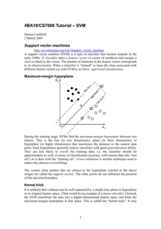
1. 4BA10/CS7008 Tutorial – SVM
Darren Caulfield
2 March 2009
Support vector machines
http://en.wikipedia.org/wiki/Support_vector_machine
A support vector machine (SVM) is a type of classifier that became popular in the
early 1990s. A classifier takes a feature vector (a vector of numbers) and assigns a
class (a label) to the vector. The number of elements in the feature vector corresponds
to its dimensionality. When a classifier is “trained” to learn the class associated with
different feature vectors (as with SVMs), we have supervised classification.
Maximum-margin hyperplane
During the training stage, SVMs find the maximum-margin hyperplane between two
classes. This is the line (in two dimensions), plane (in three dimensions) or
hyperplane (in higher dimensions) that maximises the distance to the nearest data
point. Such hyperplanes generally lead to classifiers with good generalisation ability.
They are less likely to overfit the training data, i.e. the classifier should do
approximately as well, in terms of classification accuracy, with unseen data (the “test
set”) as it does with the “training set”. Cross-validation is another technique used to
reduce the chances of overfitting.
The vectors (data points) that are closest to the hyperplane (circled in the above
image) are called the support vectors. The other points do not influence the position
of this decision boundary.
Kernel trick
It is unlikely that a dataset can be well separated by a simple line, plane or hyperplane
in its original feature space. (That would be an example of a linear classifier.) Instead,
the SVM transforms the data into a higher-dimensional feature space and finds the
maximum-margin hyperplane in that space. This is called the “kernel trick”. It only
1

2. requires the specification of a function – the kernel – that returns the distance between
any 2 points in the hyperspace.
The most popular kernels are listed below, with the parameter names that are used by
both LIBSVM and OpenCV. Custom kernels can significantly improve classification
accuracy, however. For example, we could define a string kernel for DNA sequences.
Linear: no mapping is done, linear discrimination (or regression) is done in the
original feature space. It is the fastest option.
d(x,y) = x•y == (x,y)
Poly: polynomial kernel:
d(x,y) = (gamma*(x•y)+coef0)degree
RBF: radial-basis-function kernel; a good choice in most cases:
d(x,y) = exp(-gamma*|x-y|2)
Sigmoid: sigmoid function is used as a kernel:
d(x,y) = tanh(gamma*(x•y)+coef0)
Soft margin SVM
Even with the kernel trick, some datasets are not perfectly separable, either because
the features do not discriminate between the classes well enough or because some
data points have been mis-labelled. “Soft margin” SVMs find hyperplanes that split
the data as cleanly as possible, while allowing some examples to remain on the wrong
side of the hyperplane.
OpenCV implementation
The Machine Learning library in OpenCV 1.0 implements several types of classifier,
including SVMs. However, very little SVM sample code is available to date. The
documentation can be found here:
http://opencvlibrary.svn.sourceforge.net/viewvc/opencvlibrary/trunk/opencv/d
oc/ref/opencvref_ml.htm
The functionality closely mirrors that of the more mature LIBSVM (see below).
Other classifiers to be found in OpenCV include: Bayes Classifier, k Nearest
Neighbours, Decision Trees, Boosting, Random Trees, Expectation-Maximization and
Neural Networks.
Evaluation
Classifiers often have their accuracy evaluated in terms of true positives and false
positives for a given threshold:
or by plotting true positives versus false positives while changing some threshold – a
receiver operating characteristic (ROC curve).
2

3. The importance of features
Much of the research literature is concerned with the accuracy of various classifiers,
often benchmarked against various standard datasets. It is important to realise that the
best way to “solve” a classification problem (or at least improve the accuracy) is to
find, extract or develop better features. With discriminative features a “basic”
approach, e.g. Naïve Bayes or k Nearest Neighbour, will usually do as well as an
advanced approach. No classifier will ever be accurate with weak features.
Tutorial tasks
Download and unzip LIBSVM and the other associated files:
https://www.cs.tcd.ie/Darren.Caulfield/vision
Further information: “Chih-Chung Chang and Chih-Jen Lin, LIBSVM: a library for
support vector machines”, 2001. The software is available at
http://www.csie.ntu.edu.tw/~cjlin/libsvm
svm-toy
Navigate to the “windows” folder and run “svm-toy.exe”. Load the data file
“fourclass_rescaled_for_app.txt”. (It is actually only a two-class dataset, adapted from
the LIBSVM dataset page.)
Here is the LIBSVM parameters guide (compare to the kernels listed above):
-s svm_type : set type of SVM (default 0)
0 -- C-SVC
1 -- nu-SVC
2 -- one-class SVM
3 -- epsilon-SVR
4 -- nu-SVR
-t kernel_type : set type of kernel function (default 2)
0 -- linear: u'*v
1 -- polynomial: (gamma*u'*v + coef0)^degree
2 -- radial basis function: exp(-gamma*|u-v|^2)
3 -- sigmoid: tanh(gamma*u'*v + coef0)
-d degree : set degree in kernel function (default 3)
-g gamma : set gamma in kernel function (default 1/k)
-r coef0 : set coef0 in kernel function (default 0)
-c cost : set the parameter C of C-SVC, epsilon-SVR, and nu-SVR (default 1)
-n nu : set the parameter nu of nu-SVC, one-class SVM, and nu-SVR (default 0.5)
-p epsilon : set the epsilon in loss function of epsilon-SVR (default 0.1)
-m cachesize : set cache memory size in MB (default 100)
-e epsilon : set tolerance of termination criterion (default 0.001)
-h shrinking: whether to use the shrinking heuristics, 0 or 1 (default 1)
-b probability_estimates: whether to train a SVC or SVR model for probability estimates, 0 or
1 (default 0)
-wi weight: set the parameter C of class i to weight*C, for C-SVC (default 1)
The k in the -g option means the number of attributes in the input data.
option -v randomly splits the data into n parts and calculates cross
validation accuracy/mean squared error on them.
Click “Run” with the default parameters left unchanged and observe the classification
result.
3

4. Change the parameters (in the text box at the bottom right). In particular, try changing
the t, c g, d and r values. Find parameters that leave the two classes well separated.
svm-train and svm-predict
Download and unzip the “a1a” dataset (training and test sets) and put the files in the
“windows” folder of LIBSVM. Open a command prompt in that folder.
Usage: svm-train [options] training_set_file [model_file]
Usage: svm-predict [options] test_file model_file output_file
Run the following commands. The train a classifier (on the training set) using a RBF
kernel (default), and use it for prediction (classification) on the test set:
svm-train.exe -c 10 a1a.txt a1a.model
svm-predict.exe a1a.t a1a.model a1a.output
Change the –c parameter from 0.01 to 10000 (increase by a factor of 10 each time)
and study the effect.
Change the –g (gamma) parameter.
This training set is unbalanced: there are 1210 examples from one class and 395
examples from the other. Try the “–w1 weight” and “–w-1 weight” options to adjust
the penalty for misclassification.
See the following page for some 3D results:
http://www.csie.ntu.edu.tw/~cjlin/libsvmtools/svmtoy3d/examples/
4