1. 66//1010//20132013
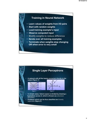
Training in Neural Network
• Learn values of weights from I/O pairs
• Start with random weights
• Load training example’s input
• Observe computed input
• Modify weights to reduce difference
• Iterate over all training examples
• Terminate when weights stop changing
OR when error is very small
Single Layer Perceptrons
• A network with all the inputs connected directly to the
output (figure 1)
• In simple cases, feature space is divided by drawing a
hyperplane across it, which is Known as a decision
boundary
• Problems which can be thus classified are linearly
separable (figure 2)
++
++
++
++ --
--
--
--
xx11
xx22
FigureFigure 11 FigureFigure 22

2. 66//1010//20132013
Single Layer Perceptrons
• Classical Measure of Error
– Squared error
– Where Err is the difference between the target value
and the output by the network
• Weight Modifying
– Use gradient descent to reduce the squared error by
calculating the partial derivative of E with respect to
each weight
j
jj
xinfErr
Err
Err
E
*** )('−=
∂
∂
=
∂
∂
ww
: Learning Rate: Learning Rate
Error Back-Propagation
The gradient descent
• The gradient of the error E gives the direction
where the error function at the current setting of
the w will increase. In order to decrease E, we
take a small step in the opposite direction, -G

3. 66//1010//20132013
Error Back-Propagation
The gradient descentThe gradient descent
InIn 22D (one weight)D (one weight)
By repeating this over and over, we moveBy repeating this over and over, we move
"downhill" in"downhill" in EE until we reach a minimumuntil we reach a minimum
Error Back-Propagation
The gradient descentThe gradient descent

4. 66//1010//20132013
Single Layer Perceptrons –
a basic application
• Suppose we have data about the height and
the age of a population of 100 people.
• So we can plot a 2D sketch (x is the age, y
the height)
• How can we predict the height of a 101th
person, given his age?
UsingUsing aa modelmodel of the data. The simplestof the data. The simplest
model can be :model can be : y = wy = w11 x + wx + w00
This may exactly be the equation of theThis may exactly be the equation of the
output of a neuron networkoutput of a neuron network
Different Non-Linearly
Separable Problems
StructureStructure
ExclusiveExclusive--OROR
ProblemProblem
Classes withClasses with
Meshed regionsMeshed regions
Most GeneralMost General
Region ShapesRegion Shapes
SingleSingle--LayerLayer
TwoTwo--LayerLayer
ThreeThree--LayerLayer
AA
AABB
BB
AA
AABB
BB
AA
AABB
BB
BB
AA
BB
AA
BB
AA

5. 66//1010//20132013
Multilayer Perceptrons(MLP)
HiddenHidden LayerLayer
Output LayerOutput Layer
AdjustableAdjustable
wweightseights
IntputIntput LayerLayer
AdjustableAdjustable
wweightseights
InputInputUnitUnits(ExternalStimuli)s(ExternalStimuli)
OutputValuesOutputValues
Types of Layers
• Input layer (units)
– Introduces input values into the network
– No activation function or other processing
• Hidden layer(s)
– Perform classification of features
– Two hidden layers are sufficient to solve any problem
– Features imply more layers may be better
• Output layer
– Functionally just like the hidden layers
– Outputs are passed on to the world outside the neural
network

6. 66//1010//20132013
MLP Characteristics
• Input propagates in a forward direction,
layer-by-layer basis
– also called Multilayer Feedforward Network, MLP
• Non-linear activation function
– differentiable
– nonlinearity prevent reduction to single-layer perceptron
• One or more layers of hidden neurons
– progressively extracting more meaningful features from
input patterns
• High degree of connectivity
Problems of MLP
• Nonlinearity and high degree of connectivity
makes theoretical analysis difficult
• Output vector rather than a single output value
• Error at output layer is clear, but error at the
hidden layers seems mysterious
• Learning process is hard to visualize
• So, Error Back-Propagation Algorithm (BPA) is
a computationally efficient training for MLP