PARTICE MOTION OF A CHARGE PARTICLE

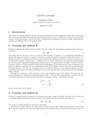
1. Particle motions
Madhurjya P Bora
Physics Department, Gauhati University
August 21, 2013
1 Introduction
The motion of a charged particle in electric and magnetic fields can be quite complicated, which needs a systematic
study. The understanding of the motion of a single charged particle in an e.m. field is key to unravel the mysteries of
complex systems like plasmas. Toward this goal, we shall begin by studying the motion of a single charged particle
of charge q in different electric and magnetic fields.
2 Constant and uniform E
Consider a constant and uniform electric field E. The force exerted by this field on a charged particle of charge q
is given by,
FE = qE: (1)
This shows that the direction of force is along the field (parallel) or opposite to it (antiparallel) depending on
whether the charge q is positive or negative. As this force pushes the particle irrespective of its initial velocity, it is
bound to accelerate it and change the kinetic energy of the particle. However, the increase of kinetic energy can not
be infinite! For example, one may argue — suppose I create an electric field between two infinitely separated points
(say by putting the oppositely charged plates infinitely apart). A charged particle of charge q placed in between
the plates will get accelerated toward the either plates (depending on q) and will continue to get accelerated as the
plates are infinitely separated. So, the charged particle may attain infinite velocity (of course non-relativistically
speaking)! However, note that the strength of the electric field also decreases as the distance between the plates
is increased which causes the initial acceleration to be very less and will thus prevent the particle from attaining
infinite velocity.
Naturally, the maximum velocity depends on the initial potential energy of the particle. We know that the
electric field E can be expressed in terms of potential as E = r. So, the maximum kinetic energy the particle
can obtain is given by q, which also gives us a limit of maximum velocity v, the particle can have,
1
2
mv2 = q;
) v =
2q
m
; (2)
where m is the mass of the particle.
3 Constant and uniform B
Consider a charged particle of charge q in a constant and uniform magnetic field B. We know that the force due
to a magnetic field is perpendicular to the velocity of the particle and the field itself and is given by,
FB = q(v B): (3)
The result is a circular motion (we shall prove that latter)
Now there are certain things to be noted. First, note that the force FB is always perpendicular to both v and
B, so the force itself can not make any displacement of the particle along its direction and the kinetic energy of
1

2. r v = v?
q
B
Figure 1: Motion of a charged particle in a magnetic field.
the particle must remain constant. We can prove it by finding out W, the work done by the field on the charged
particle, which will come out as zero,
W = FB s; (4)
where s is the displacement caused by the force,
W = FB
dv
dt
;
= q(v B)
dv
dt
= 0; (5)
as the vector dv=dt and v has same directions. As the net work done by the magnetic field is zero, it can not
change the kinetic energy of the particle and the effect of the force will be limited only to change the direction of
the particle only, which however causes an acceleration.
We can also view this circular motion from a different angle and come to the same conclusion. Look at the
Fig.1. As the particle moves in a circular orbit, the instantaneous force on the particle, which is given by Eq.(3) is
definitely not zero. However, the net force on the particle over a full period of revolution is zero. We can prove it
by considering the magnitude of the force FB,
FB = qvB sin : (6)
The net force on the charged particle is an integration of FB over a full cycle, from = 0 to 2,
Net Force =
2
0
FB d; (7)
= qvB
2
0
sin d = 0:
As the net force is zero, the kinetic energy can not change.
3.1 Equation of motion
We are now in a position to mathematically describe the motion of the charged particle in a constant and uniform
magnetic field B. Consider the equation of motion for the particle (Newton’s second law),
m
dv
dt
= q(v B): (8)
It is good idea now to fix our preferred geometry. We shall consider Cartesian co-ordinates and let the direction of
B be along the z-axis, i.e. B B^z. The components of Eq.(8) are now,
m
dvx
dt
= qvyB; (9)
2

3. m
dvv
dt
= qvxB; (10)
m
dvz
dt
= 0: (11)
The third equation immediately tells us that the velocity of the particle along the magnetic field i.e. vz is constant.
In order to solve the other two components, we take a time derivatives of Eq.(9),
m
d2vx
dt2 = qB
dvy
dt
: (12)
Substituting now for dvy=dt from Eq.(10), we get,
d2vx
dt2 = !2vx; (13)
where ! = qB=m has the dimension of frequency. The most general solution of the above equation is,
vx = v0e(i!t+); (14)
which, without loss of any generality can be written as,
vx = v0ei!t: (15)
Note that as the magnetic field can not change the magnitude of the total velocity, v2 = v2x
y + v2
z , the sum of
+ v2
v2x
and v2
y must be constant as vz is constant. Denoting now,
v? =
q
v2x
y; (16)
+ v2
we can write Eq.(15) as,
vx = v?ei!t: (17)
We can now derive the expression for vy by using the above expression in Eq.(9),
vy = iv?ei!t: (18)
Ever wondered, why we had to find the above expression to derive an expression for vy by using Eq.(17)? The
answer is that both vx;y are related to each other through the relation (16). A change in vx must be reflected in
an opposite change in vy and vice versa. If we had found the relations for vx;y independently, then we would loose
this dependence!
3.2 Orbit
We can now find out the equation of the orbit of the charged particle by integrating Eqs.(17,18) with respect to
time [note that vx;y = (x_ ; y_)],
x = irLei!t + x0; (19)
y = rLei!t + y0; (20)
where rL = v?=! has the dimension of length. Extracting the real parts of Eqs.(19,20), we get,
(x x0)2 + (y y0)2 = r2L
; (21)
which is an equation of circle centred at (x0; y0) with a radius rL. This gyrating motion is known as Larmor gyration
and the radius rL is known as Larmor radius. The frequency of gyration is ! is known as gyro-frequency. The
centre of the orbit (x0; y0) is known as the guiding centre for the orbit of the charged particle. . We can now talk
about the direction of motion of the charged particle in the orbit for positive and negative charges. What governs
this? At this moment, it is helpful to remember Fleming’s left hand rule which tells us that a charged particle
moves in a magnetic field in such a way so that the magnetic field generated by the flow of the current (movement of
charged particle creates current) always opposes the external magnetic field. So, an electron moves in the clockwise
3

4. rL
v?
q = e+
B
rL v?
q = e
B
Figure 2: Directions of gyrations of an electron and an ion around a magnetic field.
direction as seen from the top in a magnetic field coming out of the paper and an ion moves anti-clockwise (see
Fig.2).
However, it is also useful to look this phenomena from the point of view of conservation of energy. Assume that
the magnetic field created by the movement of a charged particle is along the same direction as the external magnetic
field B. In such case, the strength of the magnetic field will increase which will further cause the charged particle
to rotate rapidly in a tighter orbit. This in turn will cause more generation of current and thus more magnetic field
and the process feedbacks on itself resulting generation of a magnetic field of arbitrarily large strength and infinite
velocity, which simply violates the conservation of energy. Hence Fleming’s rule!
4 Drifts
Drifts are secondary motions of charged particle in electromagnetic fields apart from its primary motion of gyration.
One can have several drifts at the same time and it all depends on geometry and configuration of the fields involved.
4.1 Electric or E B drift
This drift arises due to combined action of an electric and magnetic field. Consider now a situation where a uniform
and constant magnetic field of strength B is along the z-axis and being superimposed with a constant and uniform
electric field E, which is along the y-direction (see Fig.3). The components of equation of motion for the charged
z
y
x
B = B^z
E = E^y
Figure 3: A combined E and B field.
4

5. y
x
B
z
E
q = e+
vEB
q = e
Figure 4: E B drift of charged particles.
particle are,
m
dvx
dt
= qvyB; (22)
m
dvy
dt
= qE qvxB; (23)
m
dvz
dt
= 0: (24)
0x
From which we can see that the component of velocity along the magnetic field is constant i.e. vz is constant. As
the fields are constants, we make a scale transformation by defining new velocity vin place of vx as,
v0x
= vx
E
B
; (25)
which transforms Eqs.(22,23) as,
m
dv0x
dt
= qvyB; (26)
m
dvy
dt
= qv0x
B: (27)
Note that Eqs.(26,27) are exactly similar to Eqs(9,10) except the fact that vx is replaced by v0x
. So, the corresponding
solutions should also be valid. In other words, the solutions of Eqs.(26,27) are given by, by,
v0x
= v?ei!t; (28)
vy = iv?ei!t : (29)
Back substituting the transformation, we have,
vx = v?ei!t +
E
B
: (30)
This equation, combined with Eq.(29) completes our solutions. Note that the parts of the solution with the
exponential terms actually describes the circular motion which we have already encountered. The other part
describes a linear motion in the postive x direction. Note that the resultant linear motion, which is our drift is
independent of the charge and mass of the particle, which means both +ve and ve particles drift with the same
velocity E=B in the positive x direction. This drift is also perpendicular to both E and B. So, the combined
motion looks something like shown in Fig.4.
4.2 General expression for drift
Consider the general equation of motion of the charged particle in a combined E and B field, which is given by,
m
dv
dt
= qE + q(v B): (31)
5

6. Lets now carry out a ‘’ product of this equation with B, which results in,
m
d
dt
(v B) = q(E B) + qB(v B) qB2v: (32)
Note the above equation describes the full motion of a charged particle under the combined action of the electro-magnetic
field, which includes the circular motion (Larmor gyration) and the linear drift motion. So, we can write
the total velocity v as a combination of both,
v = vcirc + vlin; (33)
so that Eq.(32) becomes,
m
d
dt
(vcirc B) = q(E B) qB2(vcirc + vlin); (34)
as the vlin = E=B is a constant quantity perpendicular to the magnetic field. If we now extract the component of
the equation which is parallel to vlin, we get,
vlin vEB =
E B
B2 ; (35)
which is nothing but our drift velocity vEB.
We now note that the electric field exerts a force (qE) on the charged particle, which causes the drift. So, if we
replace this force by an equivalent arbitrary force F = qE, we then have a general expression for the drift velocity
of a charged particle in a magnetic field which is acted upon by an arbitrary force field F,
vF =
1
q
F B
B2 : (36)
5 What is the origin of drift?
The drift motion of a charged particle in a magnetic field is caused by a force which does not vanish over a full
Larmor cycle of the particle around a magnetic line of the field. In other words, if there is a non-zero average force
on a charged particle in a magnetic field, we shall have a drift. This drift is always perpendicular to the magnetic
field and the direction of the non-zero average force. In the case of (E B) drift, this non-zero average is force
is provided by the electric field E. So, in principle, if we apply any other non-zero average force like gravity to a
charged particle in a magnetic field, we must have a corresponding drift.
5.1 Drift due to gravity
Consider a situation where a charged particle of charge q and mass m is subjected to move under the influence
of a gravitational field in the presence of a magnetic field of strength B. If the acceleration due to gravity of the
gravitational field is g, then the force due to gravity is Fg = mg, so that the corresponding drift is,
vg =
m
q
g B
B2 ; (37)
which we have obtained from Eq.(36). However, please note that this drift due to gravity is dependent on both mass
and charge unlike the electric drift vEB. Which means that due to gravity drift, the charged particles of opposite
signs drift in opposite directions, which in turn causes a polarisation. This polarisation of charged particles results
a secondary electric field, which can further interact with the magnetic field to cause a secondary electric drift. So,
the motion of a charged particle in different situations may get quite complicated.
6 Nonuniform B
6.1 Radius of curvature drift
Assume now that we have created a curved magnetic field, bent into a circle of radius R. As the charged particle is
tied to the magnetic field line through Larmor gyration, it must travel along the magnetic field line in a curved path,
6

7. R
B
vk
q
Fcf
Figure 5: A charged particle in a curved magnetic field.
with velocity vk, parallel to the magnetic field. Thus, the charged particle also experiences a non-zero centrifugal
force Fcf due the motion along a curved field (see Fig.5),
Fcf =
mv2
k
R2 R: (38)
This force pushes the particle in the outward direction and causes a drift,
vR =
mv2
k
q
R B
R2B2
: (39)
This drift, like the gravitational drift causes charge polarisation and thus causes a secondary electric drift.
In order to find the direction of this drift, it is important to fix an appropriate coordinate system. In this case,
we shall use a cylindrical coordinate system with the z axis coming out of the paper. The azimuthal angle is in
the direction of B and the radius vector r is in the direction of R. So, in this system, we have,
B = B ^ ; R = R^r; (40)
^
so that the direction of our drift is in the positive +z direction for positive charge and negative z direction for
negative charge. Note that in a (r; ; z) cylindrical coordinate system, ^r = ^z.
6.2 Gradient of B drift
6.2.1 Gradient in a curved magnetic field
There is one more drift associated with this radius of curvature drift vR. To see this, consider a curved magnetic
field in vacuum, as shown as in Fig.5, with the cylindrical geometry as mentioned before. In vacuum, the Ampere’s
law (Maxwell’s 4th law) becomes
r B = 0; (41)
of which in cylindrical coordinate, the components are,
(r B)r =
1
r
@Bz
@
@B
@z
; (42)
(r B) =
@Br
@z
@Bz
@r
; (43)
(r B)z =
1
r
@
@r
(rB)
1
r
@Br
@
: (44)
However, from Fig.5, we see that B has only the component, B = B ^
B ^ , and due to symmetry of the
system, there can not be any variation of the magnetic field except in the r direction. Thus, we have,
1
r
d
dr
(rB) = 0;
) B /
1
r
: (45)
7

8. So, we see that in a curved magnetic field, the magnetic field develops a gradient (becomes non-uniform) which is
directed toward the centre i.e. decreases as one goes out along the radius.
From Maxwell’s equation now, we know that a nonuniform magnetic field can accelerate charged particle and
so, we need to re-write the equation of motion of a charged particle in a nonuniform magnetic field to see, if it
results in any non-zero average force.
6.2.2 Gradient of B drift
We shall consider a situation, exactly same to the one, when we had constant and uniform magnetic field. Here, we
are going to relax one of the constraints of the magnetic field, letting it to vary in space i.e. to have a nonzero rB.
Let our magnetic field B be along the z-axis but only allow it to vary, very slowly along the y-axis. Also assume
that the variation itself is constant i.e.,
B = B(y) ^z; (46)
dB
6= 0 = constant: (47)
dy
Our equation of motion is now,
m
dv
dt
= F = q(v B); (48)
and the components are,
Fx = qvyB(y); (49)
Fy = qvxB(y); (50)
Fz = 0: (51)
So, like before, the z component of the velocity is constant as there is no force along this direction. As our B now
varies very slowly along the y direction, we can expand it in a Taylor series along y,
B(y) ' B0 + y
@B
@y

12. y=0
; (52)
where B0 is the value of the magnetic field at y = 0.
Because the variation of our B is very slow, we can in fact borrow the results from the uniform-B section
[Eqs.(17-20)] and expect that our new results should not be much different from the earlier ones. The components
of force along with the above expansion are then,
Fx = qv? sin(!t)
B0 + rL cos(!t)
@B
@y

16. y=0
#
; (53)
Fy = qv? cos(!t)
B0 + rL cos(!t)
@B
@y

20. y=0
#
: (54)
Note that we have taken only the real parts of Eqs.(17-20). In order to determine, whether these forces are nonzero
when averaged over a full Larmor gyration, we need to take an angular average of both Fx;y over a full period,
hFx;yi =
1
2

21. Fx;y d; d d(!t): (55)
Due the sines and cosines, we see that only hFyi is nonzero and is given by,
hFyi =
1
2
qv?rL
@B
@y

25. y=0
: (56)
Note that
cos2
= 1=2. So, we conclude that due the gradient of the magnetic field in the y direction, we have a
net nonzero force along the y-axis and so should give rise to a drift,
vrB =
1
2
v?rL
@B
@y

29. y=0
^y B
B2 : (57)
8

30. Writing ^y(@B=@y)jy=0 as rB, we can rearrange the above expression as,
vrB =
1
2
v?rL
B rB
B2 : (58)
It is customary to write frequency ! as always a positive quantity by expressing it as ! = jqjB=m, so that we can
write the final expression for vrB as,
vrB =
1
2
v2?
!
B rB
B2 : (59)
6.3 Combined vR and vrB
We have seen now that due to the curvature of the magnetic field, the magnetic also develops a gradient and so a
drift. This drift has to be added to the already existing radius of curvature drift to get the complete picture,
vR+rB = vR + vrB =
mv2
k
q
R B
R2B2
1
2
v2?
!
B rB
B2 :
Note that in this case, the rB is in the ^r direction so that the direction of vrB is again +z direction for positively
charged particle, which simply adds to the radius of curvature drift.
9