
Recommandé
Contenu connexe
Tendances
Tendances (20)
Similaire à Angle Modulation – Frequency Modulation Explained
Similaire à Angle Modulation – Frequency Modulation Explained (20)
Dernier
Dernier (20)
Angle Modulation – Frequency Modulation Explained
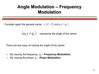
- 1. Angle Modulation – Frequency Modulation Consider again the general carrier vc ( t ) = Vc cos( ωc t + φc ) ( ωc t + φc ) represents the angle of the carrier. There are two ways of varying the angle of the carrier. • By varying the frequency, ωc – Frequency Modulation. • By varying the phase, φc – Phase Modulation 1
- 2. Frequency Modulation In FM, the message signal m(t) controls the frequency fc of the carrier. Consider the carrier vc ( t ) = Vc cos( ωc t ) then for FM we may write: FM signal v s ( t ) = Vc cos( 2π ( f c + frequency deviation ) t ) ,where the frequency deviation will depend on m(t). Given that the carrier frequency will change we may write for an instantaneous carrier signal Vc cos( ωi t ) = Vc cos( 2πf i t ) = Vc cos( φi ) where φi is the instantaneous angle = ωi t = 2πf i t and fi is the instantaneous frequency. 2
- 3. Frequency Modulation dφi 1 dφi Since φi = 2πf i t then = 2πf i or fi = dt 2π dt i.e. frequency is proportional to the rate of change of angle. If fc is the unmodulated carrier and fm is the modulating frequency, then we may deduce that 1 dφi f i = f c + Δf c cos( ωm t ) = 2π dt ∆fc is the peak deviation of the carrier. 1 dφi Hence, we have = f c + Δf c cos( ωm t ) ,i.e. dφi = 2πf c + 2πΔf c cos( ωm t ) 2π dt dt 3
- 4. Frequency Modulation After integration i.e. ∫ (ωc + 2πΔf c cos( ωm t ) ) dt 2πΔf c sin ( ωm t ) φi = ωc t + ωm Δf c φi = ωc t + sin ( ωm t ) fm Hence for the FM signal, v s ( t ) = Vc cos( φi ) Δf c v s ( t ) = Vc cos ωc t + sin ( ωm t ) fm 4
- 5. Frequency Modulation Δf c The ratio is called the Modulation Index denoted by β i.e. fm Peak frequency deviation β= modulating frequency Note – FM, as implicit in the above equation for vs(t), is a non-linear process – i.e. the principle of superposition does not apply. The FM signal for a message m(t) as a band of signals is very complex. Hence, m(t) is usually considered as a 'single tone modulating signal' of the form m( t ) = Vm cos( ωm t ) 5
- 6. Frequency Modulation Δf The equation v s ( t ) = Vc cos ωc t + c sin ( ωm t ) may be expressed as Bessel fm series (Bessel functions) ∞ v s ( t ) = Vc ∑ J ( β ) cos( ω n c + nωm ) t n= −∞ where Jn(β) are Bessel functions of the first kind. Expanding the equation for a few terms we have: v s (t ) = Vc J 0 ( β ) cos(ω c )t + Vc J 1 ( β ) cos(ω c + ω m )t + Vc J −1 ( β ) cos(ω c − ω m )t Amp fc Amp fc + fm Amp fc − fm + Vc J 2 ( β ) cos(ω c + 2ω m )t + Vc J − 2 ( β ) cos(ω c − 2ω m )t + Amp fc +2 fm Amp fc −2 f m 6
- 7. FM Signal Spectrum. The amplitudes drawn are completely arbitrary, since we have not found any value for Jn(β) – this sketch is only to illustrate the spectrum. 7
- 8. FM Signal Waveforms. If we plot fOUT as a function of VIN: In general, m(t) will be a ‘band of signals’, i.e. it will contain amplitude and frequency variations. Both amplitude and frequency change in m(t) at the input are translated to (just) frequency changes in the FM output signal, i.e. the amplitude of the output FM signal is constant. Amplitude changes at the input are translated to deviation from the carrier at the output. The larger the amplitude, the greater the deviation. 16
- 9. FM Signal Waveforms. Frequency changes at the input are translated to rate of change of frequency at the output.An attempt to illustrate this is shown below: 17
- 10. Significant Sidebands – Spectrum. As shown, the bandwidth of the spectrum containing significant components is 6fm, for β = 1. 23
- 11. Carson’s Rule for FM Bandwidth. An approximation for the bandwidth of an FM signal is given by BW = 2(Maximum frequency deviation + highest modulated frequency) Bandwidth = 2(∆f c + f m ) Carson’s Rule 25
- 12. Narrowband and Wideband FM Narrowband FM NBFM From the graph/table of Bessel functions it may be seen that for small β, (β ≤ 0.3) there is only the carrier and 2 significant sidebands, i.e. BW = 2fm. FM with β ≤ 0.3 is referred to as narrowband FM (NBFM) (Note, the bandwidth is the same as DSBAM). Wideband FM WBFM For β > 0.3 there are more than 2 significant sidebands. As β increases the number of sidebands increases. This is referred to as wideband FM (WBFM). 26
- 13. Comments FM • The FM spectrum contains a carrier component and an infinite number of sidebands at frequencies fc ± nfm (n = 0, 1, 2, …) ∞ FM signal, v s (t ) = Vc ∑J n = −∞ n ( β ) cos(ω c + nω m )t • In FM we refer to sideband pairs not upper and lower sidebands. Carrier or other components may not be suppressed in FM. • The relative amplitudes of components in FM depend on the values Jn(β), where α Vm β= thus the component at the carrier frequency depends on m(t), as do all the fm other components and none may be suppressed. 28