Empirical investigation of government expenditure and revenue nexus; implication for fiscal sustainability in nigeria

Journal of Economics and Sustainable Development www.iiste.org
ISSN 2222-1700 (Paper) ISSN 2222-2855 (Online)
Vol.4, No.9, 2013
135
Empirical Investigation of Government Expenditure and Revenue
Nexus; Implication for Fiscal Sustainability in Nigeria
Matthew Abiodun Dada*
PGS Department of Economics, Faculty of Social Sciences Obafemi Awolowo University, Ile-Ife
Nigeria
* E-mail of the corresponding author: mattabey@yahoo.com
Abstract
The study attempted to find out if a long-run relationship exists between government expenditure and revenue. It
also explored the direction of causality between the government expenditure and revenue growth. These were
with a view to examining the nexus between government expenditure and revenue growth in Nigeria between
1961-2010.
The study employed econometric techniques such as unit root tests, cointegration test, error correction
mechanism and Granger causality tests. Times series data covering the period (1961-2010) on such variables as
government expenditure, government revenue and real GDP were sourced from CBN Statistical Bulletin (2010)
Edition, augmented with CBN Annual Report and Statement of Accounts (Various Years) and World
Development Indicators (WDI) of the World Bank’s CD-ROM.
The results from ADF and PP unit root tests show that both government expenditure and revenue are I(1) process.
The two variables became I(0) after taking their first differences. Also, the results obtained from Engle-Granger
and Johansen methods of cointegration tests indicate that there was no long-run relationship between
government expenditure and revenue in Nigeria during the period under investigation. The result of the error
correction model of government spending confirmed the non-existence of long-run relation between expenditure
and revenue. The ECM coefficient is significant and positively signed showing that instead of convergence
relationship, there was evidence of a divergence relationship (ECM coefficient=0.368; t=3.636; p<0.01).
Similarly, the result of the error correction model of government revenue provided no evidence in support of
long-run relationship between revenue and expenditure. The ECM coefficient is significant and positively signed
showing that instead of a convergence relationship, there was evidence of a divergence relationship between
government revenue and government expenditure (ECM coefficient=0.297; t=2.620; p<0.01). The study further
conducted Granger causality tests, for the three lags used by this study, there was no causality, one-way or two-
way between government expenditure and revenue invalidating spend-revenue as well as revenue-spend
hypotheses. It rather provides evidence in support of institutional separation hypothesis. This implies that
government decision to spend as well as government decision to raise revenue is independent of each other. The
decisions on these two fiscal variables are made with no consideration for each other.
The finding of this study has a serious implication on fiscal sustainability in Nigeria. Government spending
should be based on revenue yields to reduce large fiscal deficits that are unsustainable to economic growth in
Nigeria. The study concluded that institutional separation hypothesis holds in Nigeria during the period under
investigation.
Keywords: Fiscal sustainability, Cointegration, Convergence, Divergence, Long-run relation
1. Introduction
The question of whether government expenditure growth is a driving force to increased government revenue or
otherwise has remained unresolved in the public finance literature. The fact remains that no concensus has been
reached by scholars of different ages across the globe on the direction of causality between government
expenditure and revenue. The findings of many empirical studies on this topical issue differ across countries and
economies. While fiscal synchronization hypothesis holds in some economies, it fails to hold in other economies.
Government decision on these two fiscal variables has an important timing consideration. Does government has
to raise revenue first and then spend or spend first and then raise revenue to offset the fiscal imbalances initially
created as a result of increased spending above the revenue generating capacity of the economy?. Is revenue
decision of government independent of her spending decisions? Understanding the relationships between these
two fiscal variables form an essential aspect of fiscal policy formulation and strategization. For instance, among
countries who run huge fiscal imbalances such as Nigeria, it might contribute to the formulation of specific
policies with regard to demand management. Theoretically, causality between government expenditure and
revenue are associated with different schools of Thought. There is divergence of opinions as regard the direction
of causality between the two fiscal variables.
To Keynes and the Keynesians, government should spend first and then raise revenue in order to balance what
could be referred to as fiscal equation. This view is based on the theory of compensatory finance, where fiscal

Vol.4, No.9, 2013
136
deficits are created to boost economic growth. Subsequently, through an in-built mechanism, the multiplier effect
of budget would eliminate any output gap and ensure a higher tax base, from which the extra tax revenue would
be generated to pay off for the initially created fiscal deficit.
To the Classical economics, budget must always balance. Government expenditure must not exceed its revenue.
This school of thought believes in what is known as fiscal neutrality. They are of the view that any mismatch
between government expenditure and revenue could harm the workings of the economy. It could have
distortionary effects on the smooth operation of the price system. Hence, fiscal neutrality in this context dictates
a tax and then spend paradigm. It is clearly understood that this view stands an opposing end to that of the
Keynesian. What mediates both of these extremes is the fiscal syncronisation hypothesis, a situation in which the
motivation to raise revenue and to spend is determined simultaneously (see Brown and Jackson, 1991), Lindahl
(1958) and Musgrave (1966).
Empirical studies exploring the direction of causality between government expenditure and revenue include
Peacock and Wiseman (1979), Gounder et al., (2007), Bohn (1991), Mount and Sowell (1997), Garcia and Henin
(1999), Hoover and Sheffrin (1992), Eita and Mbazima (2008) and Owoeye (1995). To the best of the author’s
knowledge, empirical studies on the relationship between government expenditure and revenue via the real
output growth using error correction modelling technique within the time frame of 1961 to 2010 are scarce for
Nigeria, hence the need for this study.
The rest of this paper is organized as follows: Section 2 discusses the theoretical and empirical literature
regarding the causal link between government revenues and expenditures. Section 3 presents the data and the
econometric methodology, Section 4 presents results and discussion while section 5 concludes.
2. Theoretical and empirical literature review
The causal relationship between government revenues and expenditures has motivated a vast literature both at
the theoretical and empirical level. An understanding of this causal link might contribute to the formulation of
specific policies with regard to deficits management and fiscal sustainability especially for countries running
large fiscal imbalances. The theoretical underpinnings of the causal link between government revenues and
expenditures are diverse as they are associated with different schools of economic thought.
Four main hypotheses have been advanced to characterize the causal relation between the two fiscal variables.
The first hypothesis is known as the revenue-spend hypothesis. It postulates a causal relation running from
revenue to spending. This implies that spending adjust in response to changes in revenues. This hypothesis was
initially formulated by Friedman (1978) and Buchanan and Wagner (1978), but these authors differed in their
perspectives. While Friedman (1978) argues that the causal relationship works in a positive direction, Buchanan
and Wagner (1978) postulate that the causal relationship is negative. According to Friedman, raising revenue
will lead to more government spending and hence to fiscal imbalances. Cutting revenue is, therefore, the
appropriate remedy to budget deficits.
On the contrary, Buchanan and Wagner (1978) propose an increase in revenue as remedy to deficit budgets.
Their point of view is that with a cut in revenue, the public will perceive that the cost of government
programmes has fallen. As a result they will demand for more programmes from the government which if
undertaken will result in an increase in government spending. Higher budget deficits will then be realized since
tax revenue will decline and government spending will increase.
The second view rests on the reverse causal relation, suggesting that government spend first and then increases
tax revenues as necessary to finance expenditures. This view was supported by Peacock and Wiseman (1979).
The spend-revenue hypothesis is valid when spending hikes created by some special events such as natural,
economic or political crises compel governments to increase taxes. As higher spending now will lead to higher
tax later, this hypothesis suggests that spending cuts are the desired solution to reducing budget deficits. This
hypothesis is also consistent with Barro’s (1979) view that today’s deficit-financed spending means increased
tax liabilities in the future, the gain today translates to pain tomorrow. This falls within the context of the
Ricardian equivalence proposition.
The third hypothesis known as fiscal synchronization suggests bidirectional causation between revenues and
spending (Musgrave, 1966; Meltzer and Richard, 1981). It postulates that governments take decisions about
revenues and expenditure simultaneously by analyzing costs and benefits of alternative programmes.
The fourth hypothesis emphasizes the possibility of independent determination of revenue and expenditure due
to institutional separation of allocation and taxation functions of government (Buchanan and Wagner, 1978;
Hoover and Sheffrin, 1992). Therefore, this view precludes unidirectional causation from revenue to spending or
from spending to revenue.
Many empirical studies have used Granger causality analysis to investigate the empirical validity of the above
propositions. The empirical findings vary across countries. Evidence supporting the revenue-spend hypothesis
has been found by Manage and Marlow (1986), Marlow and Manage (1987) and Bohn (1991) for the USA.

Vol.4, No.9, 2013
137
Empirical works supporting the revenue-spend hypothesis using sample from developing countries also include
Owoye (1995), Ewing and Payne (1998), Park (1998), Chang et al. (2002), Chang and Ho (2002a), Fuess et al.
(2003) and Baghestani and AbuAl-Foul (2004).
Studies providing support for spend-revenue hypothesis include Anderson et al. (1986), Von Furstenberg et al.
(1986) and Ram (1988a) for the USA; Hondroyiannis and Papapetrou (1996) and Vamvoukas(1997) for Greece;
and Dhanasekaran (2001) for India.
Evidence supporting the fiscal synchronization hypothesis was reported by Miller and Russek (1990) for the
USA; Bath et al. (1993) for India; Hasan and Lincoln (1997) for the UK; Cheng (1999) for Chile, Panama, Brazil,
and Peru. Li (2001) and Chang and Ho (2002b) for China. Ram (1988b) provides empirical evidence in support
of institutional separation hypothesis for India, Panama, Paraguay, and Sri Lanka. Hoover and Sheffrin (1992)
find evidence which is consistent with this hypothesis for the US economy. Baghestani and McNown (1994)
conclude that neither the revenue-spend nor the spend-revenue hypothesis accounts for budgetary expansion in
the United States. Instead, they show that both the expansion in revenue and spending is determined by the long-
run economic growth. On nine Asian countries, Narayan (2005) concludes in favour of the institutional
separation hypothesis for India, Malaysia, Pakistan, Thailand and Philippines. On the basis of both Johansen
procedure and Pesaran et al. bounds test, Yaya Keho (2009) found a positive long-run unidirectional causality
running from revenue to expenditure for Cote D’ivoire. This lack of consensus in the findings of the empirical
studies has motivated the author to re-examine this issue using error correction modelling technique, a
multivariate specification on Nigeria data.
3. Data and Methodology
The study begins by specifying a model showing a functional relationship between government expenditure on
one hand and government revenue as well as real gdp on the other hand. This implies that changes in
government spending might be as a result of changes in revenue as well as real gdp. This model captures the
effect of changes in government revenue on government spending via the output changes in the economy.
= , Rgdp … … … … … … … … … … … … … … … … … … … … … … … … … … … … … … … … … . … 1
Similarly, we specified a model showing a functional relationship between government revenue on one hand and
government expenditure as well as real gdp on the other hand. This implies that changes in government revenue
might be as a result of changes in government expenditure as well as real gdp. This model on its own captures
the effect of changes in government expenditure on government revenue via the output changes in the economy.
= , Rgdp … … … … … … … … … … … … … … … … … … … … … … … … … … … … … … … … … … 2
The notion that there is a long-run tendency for the public sector to grow relative to national income or vice-
versa has been an issue in economics that is rarely questioned. Thus, if the variables and are considered
as stochastic trends and if they follow a common long-run equilibrium, then these variables should be
cointegrated. According to Engle and Granger (1987), cointegrated variables must have an ECM representation.
The main reason for the popularity of cointegration analysis is that it provides a formal background for testing
and estimating short-run and long run relationships among economic variables. Furthermore, the ECM strategy
provides an answer to the problem of spurious correlation. If and are cointegrated, an ECM
representation could have the following form:
△ = + + △ + … … … … … … … … … … … … … … … … … … … … … … . 3
△ = + + △ + … … … … … … … … … … … … … … … … … . … … … … … . 4
where △ is the first difference operator, and , are error-correction terms lagged one period. The
error correction term in (3) is the lagged value of the residuals from the OLS regression of △ on
and the term in (4) corresponds to the lagged value of the residuals from the OLS regression of
on . If △ , △ , and in (3) and (4), are stationary, then it indicates that their right-hand
side must also be stationary. It is obvious that (3) and (4) is made up of a bivariate VAR in first differences
augmented by the error-correction terms and , indicating that ECM model and cointegration
are of the same representations.
However, it is possible that the relationship between and estimated from the ECM formulation (3) and
(4) could have been influenced by a third variable. The possibility of this may be explored within a multivariate
framework through the inclusion of other important variables, such as real GDP growth rate (Rgdp) or inflation
rates (CPI), which represent considerable determinants of government expenditure as well as government
revenue. Thus, the relationship between and can be examined within the following ECM representation:
△ = ! + ! "
+ ! △ + !" △ # + " … … … . . … … … … … … … … … . . … … … … . 5
△ = % + % &
+ % △ + %" △ # + & … … . . … … … … … … … … … . . … … … … … 6
where # could be the macroeconomic state of the economy as regards ()* , or inflation rates (+,- ) as ‘third’
variable, the system captures the response of and to changes in ()* , or +,- . The difference between
the ECM models (3) and (4) as well as (5) and (6) is the introduction of ()* , or +,- which alter the nature of

Vol.4, No.9, 2013
138
the model from the simple bivariate system to a multivariate system.
The study used annual data covering 1961-2010 on such variables as aggregate government expenditure,
aggregate government revenue and real GDP which were sourced from the CBN Statistical Bulletin, 2010
Edition augmented with CBN Annual Report and Statement of Accounts(Various Years) and World
Development Indicators (WDI) of the World Bank’s CD-ROM. Data were analyzed using descriptive and
econometric techniques.
4. Empirical Analysis
To test formally for the presence of a unit root for each variable in the model, Augmented Dickey-Fuller (ADF)
and Phillips-Perron (PP) tests of the type given by regression equations (7) and (8) were conducted. The ADF
test was conducted using the regression equation of the form:
△ ℎ = / + / + 0ℎ + 1 Ω3
4
56
△ ℎ 5 + 7 … … … … … … … … … … … … . . … … … … … … … 7
Where △ ℎ are the first differences of the series ℎ , k represents the lag order and t stands for time. Equation (7)
is specified with intercept term and time trend.
Phillips-Perron (PP) tests involve computing the following OLS regression:
ℎ = 9 + 9 ℎ + 9 〔; −
=
2
〕 + ? … … … … … … … … … … … … … … … … … … … … . . … … … … . 8
where 9 , 9 , 9 are the conventional least-squares regression coefficients. The
hypotheses of unit-root to be tested are H0 : 9 = 1 and H0 : 9 = 1, 9 = 0.
Akaike’s Information Criterion (AIC) is used to determine the lag order of each variable under study.
Mackinnon’s (1991) tables provide the cumulative distribution of the ADF and PP test statistics.
Tests for stationarity as revealed in Table 1 indicate that the null hypothesis of a unit root cannot be rejected for
the levels of the variables. Using differenced data, the computed ADF and PP tests suggested that the null
hypothesis could be rejected for the individual series, at the one or five percent significance level, and the
variables , , and ()* are integrated of order one, I(1).
Table 1 Result of Unit Root Tests
Variable ADF
Statistic
At Level
Mackinnon
Critical
Value (5%)
ADF Statistic
At First
Difference
Mackinnon
Critical Value
(5%)
Order of
Integration
GE -2.5962* -2.9399 -4.5286 -2.9422 I(1)
GR -0.2353* -2.9399 -4.5049 -2.9422 I(1)
Rgdp -0.7684* -2.9399 -3.6099 -2.9422 I(1)
Variable PP Statistic
At Level
Mackinnon
Critical
Value (5%)
PP Statistic
At First
Difference
Mackinnon
Critical Value
(5%)
Order of
Integration
GE -1.2070* -2.9399 -6.1968 -2.9422 I(1)
GR -2.1596* -2.9399 -6.2848 -2.9422 I(1)
Rgdp -2.5221* -2.9399 -5.2864 -2.9422 I(1)
(*) denotes rejection of the hypothesis of no unit root at the level of the variables at 5% significance level.
Results of the cointegration tests on the study variables
Having determined that the variables are stationary at first differences, the study proceeds to examine whether
the variables in question have common trends or move together over time. The employed both Engle-Granger
and Johansen cointegration techniques. Engle and Granger (1987) show that if there is a cointegrating vector, a
simple two-step residual-based testing procedure can be employed to test for cointegration. In this case, a long-
run equilibrium relationship between components of Yt can be estimated by running a regression
equation of the form:
Y1,t = βY2,t + ut …………………………………………………………………….............................(9)

Vol.4, No.9, 2013
139
where Y2,t = (Y2,t,…, Yk,t)́ is a (k – 1) x 1 vector. To test the null hypothesis that Yt is not cointegrated, we should
test whether the residual ût ~ I(1) against the alternatives ût ~ I(0). This can be done by any of the tests for unit
roots. The most commonly used is the Augmented Dickey-Fuller test with the constant term but with no time
trend. Critical values for this test are tabulated in Phillips and Ouliaris (1990) or Mackinnon (2010). The study
first conducted OLS-based regressions at the level of the variables. The result obtained is shown in Table (4a)
and Table (4b). The residuals obtained from these regressions were subjected to a unit root test. The ADF unit
root test confirmed that the residuals obtained from these regressions are non-stationary at level. The results of
the ADF unit root test on the residuals obtained from both regressions as shown in Table (4a) and Table (4b)
indicate that there exists no long-run relationship between government revenue and expenditure since
Mackinnon critical value at 5% is greater than the ADF statistics for both residuals as revealed in the result
presented in Table 4c.
Table (4a) Result of the OLS-based regressions at the level of the variables with government expenditure
as dependent variables
Dependent Variable: LOG(GE)
Method: Least Squares
Date: 08/17/12 Time: 19:08
Sample: 1961 2010
Included observations: 50
Variable Coefficient Std. Error t-Statistic Prob.
LOG(RGDP) 0.278382 0.056259 4.948253 0.0000
LOG(GR) 0.799280 0.034977 22.85175 0.0000
C -1.405500 0.334536 -4.201346 0.0001
R-squared 0.988954 Mean dependent var 10.12331
Adjusted R-squared 0.988484 S.D. dependent var 3.145961
S.E. of regression 0.337596 Akaike info criterion 0.724190
Sum squared resid 5.356635 Schwarz criterion 0.838911
Log likelihood -15.10475 F-statistic 2104.044
Durbin-Watson stat 0.845628 Prob(F-statistic) 0.000000
Table (4b) Result of the OLS-based regressions at the level of the variables with government revenue as
dependent variable
Dependent Variable: LOG(GR)
Date: 08/17/12 Time: 19:15
Sample: 1961 2010
LOG(RGDP) -0.199164 0.077905 -2.556508 0.0139
LOG(GE) 1.147819 0.050229 22.85175 0.0000
C 1.143803 0.439590 2.601979 0.0124

Vol.4, No.9, 2013
140
Table (4c) Result of the ADF unit root tests on the residuals of the OLS-based regressions at the level of
the variables
Variable ADF Statistic
At Level
Mackinnon Critical Value
(5%)
Order of Integration
ECM3
-2.803540 -2.9228 I(1)
ECM4
-2.712019 -2.9228 I(1)
(*) denotes non-rejection of the hypothesis of no unit root at level at 5% significance level
Potential problem with Engle-Granger approach is that the cointegrating vector will not involve Y1,t component.
In this case the cointegrating vector will not be consistently estimated from the OLS regression leading to
spurious results. Also if there is more than one cointegrating relation, the Engle-Granger approach can not detect
all of them. Empirical literature has it that one major weakness of Engle-Granger approach is that it can only
confirm the existence of cointegration but can not provide information on the number of cointegrating vectors in
the VAR. Hence this study proceeded by testing for cointegrating relationship using Johansen cointegration
approach. The results of the Johansen cointegration test as shown in Table 5 revealed that there is no long-run
relation between government expenditure and revenue.
Table 5: Results of Johansen Cointegration Test
Date: 08/17/12 Time: 19:21
Sample: 1961 2010
Test assumption: Linear
deterministic trend in the data
Series: LOG(GE) LOG(GR) LOG(RGDP)
Lags interval: 1 to 1
Likelihood 5 Percent 1 Percent Hypothesized
Eigenvalue Ratio Critical Value Critical Value No. of CE(s)
0.237273 17.68001 29.68 35.65 None
0.073518 4.678934 15.41 20.04 At most 1
0.020896 1.013631 3.76 6.65 At most 2
LR reject any cointegration at 5%(1%) critical level
The ECM results presented in Table 6a and 6b provided no evidence in support of long-run relation between
government expenditure and government revenue. The ECM coefficient as shown in Table 6a is significant and
positively signed showing that instead of a convergence relationship, there was evidence of a divergence
relationship between government expenditure and government revenue (ECM coefficient=0.368; t=3.636;
p<0.01). Similarly, the ECM coefficient shown in Table 6b is significant and positively signed showing that
instead of a convergence relationship, there was evidence of a divergence relationship between government
revenue and government expenditure (ECM coefficient=0.297; t=2.620; p<0.01).

Vol.4, No.9, 2013
141
Table 6a: Result of the error correction model of government spending
Dependent Variable: D(LOG(GE(-1)))
Date: 08/17/12 Time: 20:33
Sample(adjusted): 1963 2010
Included observations: 48 after adjusting endpoints
D(LOG(GR(-1))) 0.404580 0.101432 3.988680 0.0002
D(LOG(RGDP(-1))) 0.040526 0.105593 0.383794 0.7030
ECM3
(-1) 0.367510 0.101063 3.636443 0.0007
C 0.102992 0.040228 2.560213 0.0140
S.E. of regression 0.231248 Akaike info criterion -0.010999
Log likelihood 4.263978 F-statistic 8.769305
Table 6b: Result of the error correction model of government revenue
Dependent Variable: D(LOG(GR(-1)))
Date: 10/20/12 Time: 19:52
Sample(adjusted): 1963 2010
Included observations: 48 after adjusting endpoints
C 0.070705 0.053471 1.322303 0.1929
D(LOG(GE(-1))) 0.652841 0.161943 4.031305 0.0002
D(LOG(RGDP(-1))) 0.087960 0.133268 0.660022 0.5127
ECM4
(-1) 0.297449 0.113513 2.620395 0.0120
The study further conducted Granger causality tests, for the three lags used by this study, there was no causality,
one-way or two-way between government expenditure and revenue invalidating spend-revenue as well as
revenue-spend hypotheses. It rather provides evidence in support of institutional separation hypothesis. This
implies that government decision to spend is independent of her decision to raise revenue during the period
under study.
Table 6: Results of the Granger causality test between government expenditure and revenue
Null hypothesis No of
Obs
No of
lags
F-Value Prob. Decision Rule
D(LOG(GR(-1))) does not Granger Cause D(LOG(GE(-1)))
D(LOG(GE(-1))) does not Granger Cause D(LOG(GR(-1)))
47
46
45
1
1
2
2
3
3
1.97527
0.11389
1.30496
1.15177
0.94276
0.76619
0.16691
0.73736
0.28221
0.32609
0.42958
0.52010
Do not reject
Do not reject
Do not reject
Do not reject
Do not reject
Do not reject

Vol.4, No.9, 2013
142
5. Summary, Recommendations and Conclusion
The study attempted to find out if a long-run relationship exists between government expenditure and revenue in
Nigeria. It also investigated the direction of causality between government expenditure and revenue growth.
These were with a view to examining the nexus between government expenditure and revenue growth in Nigeria
between 1961 and 2010.
The study employed econometric techniques such as unit root tests, cointegration test, error correction
mechanism and Granger causality tests. Times series data covering the period (1961-2010) on such variables as
government expenditure, government revenue and real GDP were sourced from CBN Statistical Bulletin (2010)
Edition, augmented with CBN Annual Report and Statement of Accounts (Various Years) and World
Development Indicators (WDI) of the World Bank’s CD-ROM.
The results from ADF and PP unit root tests showed that both government expenditure and revenue are I(1)
process. The two variables became I(0) after taking their first differences. Also, the results obtained from Engle-
Granger and Johansen methods of cointegration tests indicate that there was no long-run relationship between
government expenditure and revenue in Nigeria during the period under investigation. This result agrees with
that obtained from the error correction models which provided no evidence in support of long-run relation
between expenditure and revenue. Also, the study found no causal evidence one-way or two-way between
government expenditure and revenue. These results imply that government decision to spend as well as
government decision to raise revenue is independent of each other. The decisions on these two fiscal variables
are made with no consideration for each other, hence the two variables failed to converge to a common
equilibrium. The finding of this study has a serious implication on fiscal sustainability in Nigeria. In an
economy characterized by high level of corruption and ineptitude, fiscal sustainability is under a serious threat.
Government spending should be based on revenue yields to reduce large fiscal deficits that are unsustainable to
long-run economic growth.
The study concluded that institutional separation hypothesis holds in Nigeria during the period under
investigation.
References
Anderson, W. Wallace, M.S. and Warner J.T. (1986). The Government Spending and Southern Economic
Journal 52(3): 630-639.
Baghestani, H. and AbuAl-Foul, B. (2004). The causal relation between government revenue and spending:
Evidence from Egypt and Jordan. Journal of Economics and Finance 28(2): 260-269.
Baldacci, E., Maria T.G, and Luiz, M. (2003), “More on the Effectiveness of Public Spending on Health Care
and Education: A Covariance Structure Model”, Journal of International Development, 15. 709-25.
Baghestani, H. McNown, R. (1994). Do revenues or expenditures respond to budgetary disequilibria? Southern
Economics Journal 61(2): 311-322.
Barro, R. and Sala-i-Martin, X. (1992). Public Finance in Models of Economic Growth. Review of Economic
Studies, 59: 645-661.
Bhatia, H. L. (1982). Public Finance. New Delhi: Vikas publishing.
Brennan, G. and Buchanan, J. (1980). “The power to tax: Analytical foundations of a fiscal Constitution”.
Cambridge: Cambridge University Press.
Brons, M, Groot, H. and Nijkamp P, (1999). Growth Effects of Fiscal Policies. Tinbergen Discussion Paper,
Amsterdam: Vrije Universiteit.
Buchanan, J.M., Wagner, R.W. (1978). Dialogues concerning fiscal religion. Journal of Monetary Economics, 4:
627-636.
Chang, T. and Ho, Y.H. (2002). Tax or spend, what causes what: Taiwan’s experience. International Journal of
Business Economics. 1(2): 157-165.
Chang, T. Liu, W.R. and Caudill, S.B. (2002). Tax-and-spend, spend-and-tax, or fiscal synchronization: New
evidence for ten countries. Applied Economics., 34. 1553-1561.
Clark, C. (1964). Taxmanship: Principles and Proposals for the Reform of Taxation, Hobart Paper, 26, Institute
of Economic Affairs, London.
Dalena, M. and Magazzino, C. (2010). Public expenditure and revenue in Italy, 1862 1993, MPRA Working
Paper, 27658, http://mpra.ub.uni-muenchen.de/27658/.
Eita, J.H. and Mbazima, D. (2008). “The Causal Relationship between Government Revenue and Expenditure in
Namibia” MPRA Working Paper, No. 9154.
Engle, R.F. Granger, CWJ. (1987). Cointegration and error correction: Representation, estimation and testing.
Econometrica. 55: 251-276.
Ewing, B. and Payne, J. (1998). Government revenue-expenditure nexus: evidence from Latin America. Journal
of Economic Development. 23: 57-69.

Vol.4, No.9, 2013
143
Folster, S. and Henrekson, M. (2001). Growth Effects of Government Expenditure and Taxation in Rich
Countries. European Economic Review. 45(8): 1501-1520.
Friedman, M. (1978). “The Limitations of Tax Limitation.” Policy Review (Summer): 7–14.
Fuess, M.S., Hou, W.J. and Millea, M. (2003). Tax or spend, what causes what? Reconsidering
Taiwan’s experience. International Journal of Business Economics, 2(2): 109-119.
Garcia, S. and Henin, (1999). Balancing budget through tax increases or expenditure cuts: Is it neutral?”
Economic Modeling 16 (4): 591–612.
Gounder, N., Narayan, P.K. and Prasad, A. (2007). “An Empirical Investigation of the Relationship between
Government Revenue and Expenditure: The Case of the Fiji Islands.” International Journal of Social Economics,
34(3): 147-158.
Granger, CWJ. and Newbold, P. (1974). Spurious Regression in Econometrics. Journal of Economics.2: 111-20.
Granger, CWJ. (1969). Investigating Causal Relations by Econometric Models and Cross-Spectral Methods,
Econometrica, 37, 424-438.
Hasan, S.Y. and Sukar, A.H. (1995). Short-run and long-run dynamics of expenditures and revenues
and the government budget constraint: Further evidence. Journal of Economics. 22(2): 35-42.
Hoover, K.D. Sheffrin, S.M. (1992). Causation, spending and taxes: Sand in the sandbox or tax collector for the
welfare state. American Economic Review, 82(1): 225-248.
Johansen, S. (1988). Statistical analysis of cointegration vectors, Journal of Economics Dynamics and Control,
12, 231-254
Jones, R and Joulfaian, D. (1991). Dynamics of government revenues and expenditures industrial economies.
Journal of Applied Economics. 23: 1839-1844.
Koren, S. and Stiassny, A. (1998). Tax and spend, or spend and tax? An international study. Journal of Policy
Modeling 20: 163-91.
MacKinnon, J.G. (2010). "Critical Values for Cointegration Tests,"Working Papers 1227, Queen's University,
Department of Economics.
Mackinnon, J.G., Haug, A.A. and Michelis, L. (1996). "Numerical Distribution Functions of Likelihood Ratio
Tests for Cointegration," G.R.E.Q.A.M. 9609, Universite Aix-Marseille III.
Manage, N. and Marlow, M.L. (1986). The causal relation between federal expenditures and receipts. Southern
Economic Journal, 52(3): 617-629.
Marlow, M.L. and Manage, N. (1987). Expenditures and receipts: Testing for causality in state and local
government finances. Public Choice, 53(3): 243-255.
Miller, S.M. and Russek, E.S. (1990). “Cointegration and Error Correction Models: The Temporal Causality
betwecn Government Taxes and Spending. Southern Economic Journal, 57: 221-29.
Mounts, W. and Sowell, C. (1997).“Taxing, Spending, and the Budget Process: The Role of Budget Regime in
the Intertemporal Budget Constraint.” Swiss Journal of Economics and Statistics. 133(3): 421–39.
Musgrave, R. A. and Musgrave, P.B. (1982). Public Finance in theory and practice, 3rd. Ed. Boston: McGraw
Hill Inc.
Narayan, P.K., Nielsen, I. and Smyth, R.(2008). Panel Data, Cointegration, Causality and Wagner’s law:
Empirical Analysis from Chinese Provinces. China Economic Review, 19: 297-307.
Owoye, O. (1995). The causal relationship between taxes and expenditures in the G7 countries: Cointegration
and error correcting models. Journal of Applied Economics 2: 19-22.
Park, W. (1998). Granger causality between government revenues and expenditures in Korea. Journal of
Economic Development, 23(1): 145-155.
Peacock, A. and Wiseman, J. (1979). Approaches to the analysis of government expenditure growth. Public
Finance Review, 7: 3-23.
Peacock, A.T. and Wiseman, J. (1961). The Growth of Public Expenditure in the United Kingdom.
Princeton N.J: Princeton University Press for the National Bureau of Economic Research.
Perron, P. (1989). The great crash, the oil price shock and the unit root hypothesis. Econometrica. 57(6): 1361-
1401.
Phillips, P. and Ouliaris, S. (1990). Asymptotic Properties of residual based test for cointegration, Econometrica
58: 73-93.
Ram, R. (1988a). Additional evidence on causality between government revenue and government expenditure.
Southern Economic Journal. 54(3): 763-769.
Ram, R. (1988b). A Multicountry perspective on causality between government revenue and government
expenditure. Journal of Public Finance. 43: 261-269.
Roman, K. (2010). “Financial Econometric with E-views “. Copy right 2010 Roman Kozhan and Ventus
Publishing APS . ISBN 978-87-7681-427-4.
Rosen, H. S. (1995). Public Finance, 4th Ed. Chicago: Richard Irwin. S71-S102.

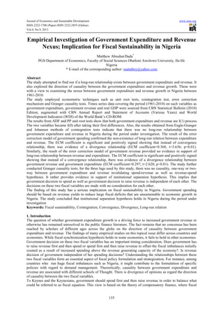
Vol.4, No.9, 2013
144
Ross, K. L. and Payne, J. E. (1998). “A Re-examination of Budgetary Disequilibria.” Public Finance Review 26
(1): 67–79.
Vamvoukas, G. (1997). Budget expenditures and revenues: An application of the error correction modeling.
Journal of Public Finance. 52(1): 139-143.
Von Furstenbeg, G.M. Green, J. and Jeong, J.H. (1986). Tax and Spend or Spend and Tax. Rev. Econ. Stat.,
68(2): 179-188.
Wagner, A. (1890). Classic in the Theory of Public Finance. London,and Macrnillan. 3rd
ed. (Leipzigt partly
reprinted in R.A. Musgrave and A.T. Peacock (l958).
Appendix A
Figure 1: Graphical Presentation of Variables in their Level form
4
6
8
10
12
14
16
65 70 75 80 85 90 95 00 05 10
LOG(GE) LOG(GR) LOG(RGDP)

Vol.4, No.9, 2013
145
Appendix B
Figure 2: Graphical Presentation of Variables at First Differences
-1.0
-0.5
0.0
0.5
1.0
1.5
2.0
65 70 75 80 85 90 95 00 05 10
D(LOG(GE(-1)))
D(LOG(GR(-1)))
D(LOG(RGDP(-1)))

Vol.4, No.9, 2013
146
Appendix C
Figure 3: Graphs of Data Residual Series
Note: ECM1 = ECM3
ECM2 = ECM4
as shown in the figure
0
2,000,000
4,000,000
6,000,000
8,000,000
65 70 75 80 85 90 95 00 05 10
AGEXP
0
1,000,000
2,000,000
3,000,000
4,000,000
65 70 75 80 85 90 95 00 05 10
AGREV
0
200,000
400,000
600,000
800,000
65 70 75 80 85 90 95 00 05 10
RGDP
-1.2
-0.8
-0.4
0.0
0.4
0.8
65 70 75 80 85 90 95 00 05 10
ECM1
-.8
-.4
.0
.4
.8
65 70 75 80 85 90 95 00 05 10
ECM2

This academic article was published by The International Institute for Science,
Technology and Education (IISTE). The IISTE is a pioneer in the Open Access
Publishing service based in the U.S. and Europe. The aim of the institute is
Accelerating Global Knowledge Sharing.
More information about the publisher can be found in the IISTE’s homepage:
http://www.iiste.org
CALL FOR PAPERS
The IISTE is currently hosting more than 30 peer-reviewed academic journals and
collaborating with academic institutions around the world. There’s no deadline for
submission. Prospective authors of IISTE journals can find the submission
instruction on the following page: http://www.iiste.org/Journals/
The IISTE editorial team promises to the review and publish all the qualified
submissions in a fast manner. All the journals articles are available online to the
readers all over the world without financial, legal, or technical barriers other than
those inseparable from gaining access to the internet itself. Printed version of the
journals is also available upon request of readers and authors.
IISTE Knowledge Sharing Partners
EBSCO, Index Copernicus, Ulrich's Periodicals Directory, JournalTOCS, PKP Open
Archives Harvester, Bielefeld Academic Search Engine, Elektronische
Zeitschriftenbibliothek EZB, Open J-Gate, OCLC WorldCat, Universe Digtial
Library , NewJour, Google Scholar

Empirical investigation of government expenditure and revenue nexus; implication for fiscal sustainability in nigeria

Recommandé

Recommandé

Contenu connexe

Tendances

Tendances (20)

En vedette

En vedette (8)

Similaire à Empirical investigation of government expenditure and revenue nexus; implication for fiscal sustainability in nigeria

Similaire à Empirical investigation of government expenditure and revenue nexus; implication for fiscal sustainability in nigeria (20)

Plus de Alexander Decker

Plus de Alexander Decker (20)

Dernier

Dernier (20)

Empirical investigation of government expenditure and revenue nexus; implication for fiscal sustainability in nigeria