1. British Actuarial Journal
http://journals.cambridge.org/BAJ
Additional services for British Actuarial
Journal:
Email alerts: Click here
Subscriptions: Click here
Commercial reprints: Click here
Terms of use : Click here
How Actuaries Can Use Financial Economics
A.D. Smith
British Actuarial Journal / Volume 2 / Issue 05 / December 1996, pp 1057 - 1193
DOI: 10.1017/S1357321700004876, Published online: 10 June 2011
Link to this article: http://journals.cambridge.org/
abstract_S1357321700004876
How to cite this article:
A.D. Smith (1996). How Actuaries Can Use Financial Economics. British
Actuarial Journal, 2, pp 1057-1193 doi:10.1017/S1357321700004876
Request Permissions : Click here
Downloaded from http://journals.cambridge.org/BAJ, IP address: 170.194.32.58 on 20 Mar 2015
2. B.A.J.2,V, 1057-1193(1996)
HOW ACTUARIES CAN USE FINANCIAL ECONOMICS
B Y A . D . SMITH, B.A.
[Presented to the Institute of Actuaries, 25 March 1996]
ABSTRACT
There has recently been some debate about the usefulness of financial economics to the actuarial
profession. The consensus appears to be that the techniques are potentially valuable, but the published
material is not quite 'oven ready'. Some development work is required before the material can be
applied.
The author has carried out much of the necessary development work on behalf of various clients
over the last few years. On some occasions the results have conflicted with more conventional
actuarial methods. The main aim of the paper is to bring the new techniques into the public domain
so that they can be properly discussed by the profession, and adopted more widely if appropriate.
The paper contains a number of worked examples using techniques developed by financial
economists. The author has listed the computer code which generated the examples and deposited
copies on the Internet, so that others can explore the issues with a minimal development overhead.
KEYWORDS
Financial Economics; Stochastic Models; Asset-Liability Studies; Dynamic Optimisation;
Equilibrium; Arbitrage; Risk-Neutral Law
1. INTRODUCTION
1.1 Financial economics is the application of economic theory to financial
markets. Its use in actuarial work continues to be controversial. At one extreme,
I have seen models applied uncritically in apparently blind faith, while at the
other extreme, some actuaries have claimed that financial economics is part of a
conspiracy to displace traditional methods with unsound practices (see, for
example, Clarkson in the discussion of Bride & Lomax, 1994).
1.2 Financial economics has produced several specific models which have
come into widespread use within the financial community. Examples include the
capital asset pricing model, or CAPM, as derived by Sharpe (1964) and the Black
& Scholes (1973) formula for option pricing. There are also a number of
established models describing the term structure of interest rates and the pricing
of associated derivatives, such as Ho & Lee (1986), Hull & White (1990) and
Black, Derman & Toy (1990). Several actuarial papers have been published
applying such models. Examples include Wilkie (1987) who applies option
pricing to bonus policy, or Mehta (1992) who, inter alia, demonstrates the use of
the CAPM to derive discount rates for calculating appraisal values.
1.3 It is not the purpose of this paper to review established models such as
the CAPM or the Black-Scholes formula. Instead, I will examine some underlying
1057
3. 1058 How Actuaries can use Financial Economics
techniques which have been fruitful in financial economics. Economists have
applied these techniques to classical economic problems in order to derive the
established models. In this paper I have applied the same techniques to some
current actuarial problems, and obtained solutions which fuse traditional actuarial
methods with powerful insights from economics.
1.4 This paper is far from comprehensive. Instead, I have concentrated on a
few concepts from economics and applied these in a series of case studies. These
are deliberately detailed and 'hands on', since I believe that it is through practical
worked examples that we can best see the point of the new techniques. In a
higher level description, it is easy to gloss over the various assumptions and
approximations which need to be made to get numerical output. Despite the many
compromises and heroic assumptions involved, I am still convinced that financial
economics can enhance the work of actuaries. Since the paper mainly consists of
worked examples, it is necessarily rather piecemeal.
1.5 The intended audience for this paper is actuaries, who are able to
appreciate the technicalities of the modelling approaches that I have described.
The profession (Nowell et ah, 1995) has described financial economics as an area
in which we may have to learn some new skills for the future. I have deliberately
concentrated on the method, so that the profession may appraise in the discussion
whether the material is sound or not. The mathematics is more involved than in
many other actuarial fields, and I accept there will be some clients for whom the
style of presentation I have adopted is totally unhelpful. Such clients have very
good reasons to employ actuaries, since they have little chance of getting the
work done in-house. The communication of complex concepts to non-
mathematicians is important, but, in my view, ease of communication is never a
good reason for using an unsound method. When the profession has reached a
consensus on method, that may be the time to start thinking about how it is to be
presented to the outside world.
1.6 The remainder of this paper is organised as follows. Section 2 examines
the actuarial appraisal value construction, in the light of financial economics. I
have considered the use of risk discount rates and locking-in adjustments in a
numerical example. Alongside this, I have used the risk neutral methodology
developed by financial economists. I demonstrate that these techniques give the
same answer, although they come from very different starting premises. Section
3 then reviews the methodology of asset-liability studies from a financial
economics perspective. We pay particular attention to the optimisation techniques
developed by financial economists, and compare these with the methods actuaries
have traditionally employed. Section 4 considers the issues of capital adequacy
and risk management, from the framework of maximising shareholder value.
Section 5 applies the theories so far developed to build a stochastic asset model.
Section 6 considers the issues which arise when we try to ascribe 'market-based'
values to entities which are not traded in a liquid market. Section 7 concludes
with some general remarks. Appendix A contains some of the more complicated
mathematics involved in optimisation. Appendix B contains some notes on
4. How Actuaries can use Financial Economics 1059
calibrating stochastic asset models. Appendix C contains the computer code I
have used to generate the examples, which is, in essence, a library of stochastic
modelling functions. I have placed demonstration spreadsheets calling these
functions on the Internet at www.actuaries.org. I have collected together some of
the technical terms in a glossary which forms Appendix D.
2. THE CONCEPT OF VALUE
2.1 The Appraised Value of a PEP
2.1.1 A large amount has been written on the subject of value, both from an
actuarial and a more general economic viewpoint. We can isolate several distinct
value concepts. The present value is the result of a discounted cash flow
calculation. The economic concept of value is the price at which an asset will
trade. An appraised value refers to the result of a calculation whose output is
intended to be consistent with economic value. The assessed value or long-term
value of an asset is an intermediate stage in actuarial pension fund calculations.
These are all distinct from the actuarial reserve concept, which is the quantity of
assets required today to meet future liabilities (with a predetermined probability).
These concepts will differ numerically because of different ways of treating risk,
different cash flow expectations or because of market inefficiencies. The purpose
of this section is to reconcile three apparently different value concepts, using the
example of a personal equity plan, or PEP. The reason for choosing a PEP is its
simplicity, in particular with regard to taxation and charging structure. In order to
make the issues more comprehensible, I have produced a numerical
demonstration rather than algebraic formulae. For typesetting convenience, all
contracts are assumed to redeem in five years' time. Some of the relevant algebra
is covered in Bride & Lomax (1994).
2.1.2 Daykin has pointed out, in the discussion of Dyson & Exley (1995),
that actuaries focus on value while financial economists focus on price. The main
actuarial objections to the use of market price is that it is ambiguous, because
market values may be volatile over time. It is not so often pointed out that
actuarial appraised values are also ambiguous. The ambiguity arises because of
the subjective judgement in the choice of basis. In the view of any one actuary,
value may be moderately stable in the short term. However, if one talks to several
actuaries in succession, one may obtain a series of 'values' which are at least as
volatile as market values, if not more so. The key question must be whether a
general disregard by actuaries of the information contained in observed prices
would have a detrimental impact on the soundness of our financial management.
One message of financial economics is that market value is of crucial importance
to virtually any financial optimisation problem.
2.1.3 By way of a concrete example, we consider the valuation of a cohort of
single premium PEP business, with five years left to maturity. The unit price is
assumed to be equal to the market value of assets less selling costs, so that the
5. 1060 How Actuaries can use Financial Economics
emerging distributable profits consist entirely of management fees less expenses.
The initial situation is as follows:
Initial units in force
Initial unit price
Annual fee
Expenses per unit
10,000
£100
£0.50
2.1.4 Future assumptions, on a best estimate basis, are as follows:
12.00%
10.00%
3.:
Earned return p.a.
Lapse rate p.a.
Expense inflation p.a.
'BE
IBE
e
BE
All policies are assumed to lapse at the end of year 5 if they have not already
done so.
2.1.5 We adopt the convention that expenses are incurred at the beginning of
the year, while fees are collected at the end. Lapses occur at the year end, after
the fees have been collected. We consider only variable expenses, so that fixed
costs are added in at a later stage of the calculation. Using the assumptions in
112.1.4, we can project the business as follows, up to the 5-year time horizon:
Policy year
Unit price brought forward
Investment return
Management fee
Unit price carried forward
Units brought forward
Lapses
Units carried forward
Fees receivable at year end
Benefits payable at year end
Expenses per unit
Expenses payable at year start
1
100.00
12.00
(1.12)
110.88
10,000
(1,000)
9,000
11,200
(110,880)
-O.500
(5,000)
2
110.88
13.31
(1.24)
122.94
9,000
(900)
8,100
11,177
(110,649)
-0.516
(4,646)
3
122.94
14.75
(1.38)
136.32
8,100
(810)
7,290
11,153
(110,419)
-0.533
(4,318)
4
136.32
16.36
(1.53)
151.15
7,290
(729)
6,561
11,130
(110,190) (1
-0.550
(4,012)
5
151.15
18.14
(1.69)
167.60
6,561
(6,561)
0
11,107
,099,604)
-0.568
(3,728)
2.1.6 We can calculate present values of these quantities using an appropriate
discount rate. One possible candidate would be the assumed rate of return on the
assets. Projecting these present values into the future, we can then obtain the
figures:
Present value of fees
Present value of expenses
1
40,225
(17,815)
2
33,852
(14,353)
3
26,737
(10,872)
4
18,792
(7,341)
5
9,917
(3,728)
In this example, and for the remainder of this section, the present value is
discounted back to the begining of the policy year, so that, for example, the right
hand column is the present value of cash flows during policy year 5 as at the start
6. How Actuaries can use Financial Economics 1061
of year 5. The left hand column is the total present value of all cash flows from
years 1 to 5 as at the start of year 1. The reader who wishes to see this in more
detail will find this worked example in SECT2.XLS on the Internet.
2.1.7 We could also calculate the present value of the policyholder benefits.
Subtracting the present value of the fees, we recover the bid value of the units.
This makes a lot of sense, as the current assets have to fund both policyholder
benefits and also the fees.
2.2 The Use of Risk Discount Rates
2.2.1 Actuaries have developed the technique of appraised value to describe
the value of a block of business to the proprietors of a financial services provider.
The underlying techniques are described in Burrows & Whitehead (1987). An
essential part of the theory asserts that the discounted cash flow valuation in
112.1.5 puts too high an economic value on the business. This can be justified by
a comparison between shareholders owning the business itself, or alternatively
purchasing the underlying investments directly. Both of these alternatives would
provide the same projected rate of return, i.e. the earned rate, on a best estimate
basis. However, ownership of the business carries additional risks above those of
the underlying investments. Particular risks would include the possibility of
heavier than expected lapses or higher than expected expense inflation. The
conclusion is that, at the prices in 112.1.5, ownership of the underlying
investments would be preferable to ownership of the business. In other words, the
discounted value in H2.1.5 is not directly comparable with the market value basis
for the underlying assets. This does not necessarily mean that the present value
calculation is pointless, but it does not tell us all that we would like to know
about shareholder value.
2.2.2 One means of adjusting for the degree of risk is to postulate a required
rate of return on the financial services business. The required rate of return, or
risk discount rate (henceforth RDR) is used to discount projected distributable
profit flows and produce a shareholder value assessment. The risk discount rate
exceeds the assumed earned rate by a margin which, in some way, reflects the
degree of additional risk assumed. Much can be said about how the price
mechanisms in the market lead to certain kinds of risks being rewarded with
higher mean returns; consideration of these issues are deferred to Section 6.
2.2.3 There are significant difficulties with discounting at a rate different
from the earned rate. If such a technique were to be applied to the underlying
assets, then this would give a value below market. This is unfortunate, since the
whole point of introducing the technique was to make the appraised value of an
enterprise more consistent with the market value of traded securities. For another
example, we could consider two PEP providers, A and B, with the same best
estimate cash flows. The difference is that B has a greater degree of uncertainty
attaching to future expenses. Under conventional methodologies, a higher risk
discount rate would be applied when valuing B than when valuing A. This has
the intended result of reducing the value of B relative to A. However, the method
7. 1062 How Actuaries can use Financial Economics
achieves this implicitly by reducing the present value of future fees, and also
reducing the present value of future expenses, but to a smaller degree. Intuitively,
we might hope, on the contrary, that an increase in perceived expense risk would
result in a larger (i.e. more negative) value being placed on future expenses while
the value of fees stays the same.
2.2.4 One solution to the problems in 112.2.3 is to apply different risk
discount rates to different components of distributable profit according to their
different risk characteristics. This has been suggested by Mehta (1992), and I
agree that this is theoretically desirable, but it does not yet seem to be widely
adopted in actuarial practice, perhaps because of potential difficulties in
communicating results to the client.
2.2.5 In our current example, an appropriate risk discount rate for valuing
fees would be in excess of the expected earned rate, thus reflecting the additional
risk in a lower value. When valuing expenses the reverse applies, since a larger
(i.e. more negative) value of expenses is cautious. We, therefore, discount future
expenses at a risk discount rate below the earned rate. The parameters I have
chosen are as follows:
Fee income RDR iq 12.93%
Expense RDR ie 8.21%
Certainly, arguments could be made in favour of other parameter values; my
arguments for using these are contained in Section 6. On one hand, it could be
argued that no risk premium is appropriate in relation to inflation, as inflation is,
in some sense, a risk-free asset. On the other hand, one could point out that the
real risk is not the underlying inflation in the economy, but rather the possibility
of some management action (or inaction) which resulted in unplanned expense
overrun. In a sense, the justification for a lower discount rate is not the variability
in the cash flows, but an unwinding of over-optimistic mean estimates. The point
is that different actuaries may interpret the discount rates differently, but they can
all agree on the answer to the calculation. We could argue that for this product
the lapse risk is negligible, because, on lapsation, it is only the bid value of units
which must be paid. However, it should also be borne in mind that adverse lapse
experience will terminate fee income which might have arisen in the future, so
that there is at least an opportunity cost to adverse lapse experience. This might
justify increasing the discount rate to allow for the risk, as I have done.
2.2.6 Some care must be applied when using risk discount rates to ensure that
the quantities being discounted are actually subject to the risks for which the
discount rate has been adjusted. In our current example, I have adopted the
convention that fees are deducted before lapses are processed, so that the fees in
the first year are not subject to lapse risk. Arguably, the fee income should,
therefore, be discounted at the earned rate during the year in which it is charged,
and at the risk discount rate in prior years. Equivalently, we can fund the fees
actuarially on an annual basis. These mean that the fees emerge as a decrease in
reserves at the start of the year rather than as a cash flow item at the year end.
8. How Actuaries can use Financial Economics 1063
Adding in the present value of expenses, we obtain the following appraised
values:
Funded value of units
Increase in reserves
Present value of earnings
Present value of expenses
Appraised value
1
990,000
(10,000)
39,644
(18,867)
20,778
2
987,941
(9,979)
33,477
(15,005)
18,472
Policy year
3
985,886
(9,958)
26,535
(11,209)
15,326
4
983,835
(9,938)
18,720
(7,457)
11,262
5
981,789
(9,917)
9,917
(3,728)
6,189
2.2.7 We can solve the equation of value to find the single risk discount rate
which, when applied to projected distributed net profit, produces the appraised
value above. This provides the following implied discount rates:
Net cash flows
Implied discount rate
1
5,000
16.70%
2
5,333
16.42%
3
5,641
16.189!
4
5,926
i 15.97%
5
6,189
We can explain the decreasing implied discount rate as follows. The effect of
lapse experience on distributable profit is geared up by virtue of the subtraction
of expenses. As the expense inflation is lower than the assumed investment
return, the extent of this gearing falls over time. The falling impact of lapse risk
is consistent with a lower risk discount rate.
2.3 Cost of Capital Adjustments
2.3.1 There are several schools of thought on how appropriate discount rates
may be derived. Traditional approaches would build a discount rate for a project
by comparison with the possible returns on alternative projects. Thornton &
Wilson (1992) examine historic asset returns in detail, and implicitly assume that
the 'best estimate' expected return on assets is an appropriate rate for discounting
the liabilities of a pension fund. By the same token, in a demutualisation of a life
office, it is sometimes suggested that policyholders would require an earned rate
in respect of the profit stream they give up. These approaches are all too often
regarded as obvious, and therefore free of assumptions which ought to be tested.
On the other hand, other asset pricing models may appear to be the consequence
of numerous dubious assumptions, and, as such, are likely to produce suspect
results. The abstract construction of a risk discount rate in excess of earned rates
may, therefore, be hard to justify, except by noting that a higher risk discount rate
adjusts appraised values in the right (i.e. downwards) direction.
2.3.2 An alternative approach is to discount cash flows at an expected earned
rate, and to adjust separately for the additional risk outside the discounted cash
flow construction. One way to adjust for the risk is to measure the possible
deviations from the best estimate projection, and to allocate capital to absorb
these possible deviations. The cost of financing this additional capital is then
applied as an adjustment to the discounted cash flow, to provide the appraised
9. 1064 How Actuaries can use Financial Economics
value. This item has been called the cost of capital adjustment, or COCA, by
Bride & Lomax (1994). This idea can also be applied to solvency measurement,
capital allocation and product pricing, as described in Hooker et al. (1996).
2.3.3 The cost of capital adjustment may be applied either as an increase in
the liabilities or as a decrease in the value of the assets. Conventionally, the
adjustment has often been applied, not to the assets forming the technical
reserves, but to those assets constituting the solvency margin. In this case, the
COCA is more commonly called a locking-in adjustment.
2.3A The first step in calculating a COCA is to determine the appropriate
amount of capital at risk from adverse fluctuations, which I have called the sum
at risk (SAR). In the case of lapse risk, all future fees, except those arising at
the end of the current year, may be forfeit to heavy lapses. The cost of financing
this capital is the risk margin between the required return and that earned on
investments. Discounting these costs at the risk discount rate for the fees gives
the COCA for the value of fee income:
Sum at risk from lapse
Annual capital cost charge
Cost of capital adjustment
Value of fees
1
30,225
(280)
(580)
39,644
2
23,873
(221)
(375)
33,477
Policy year
3
16,779
(156)
(202)
26,535
4
8,855
(82)
(73)
18,720
5
(0)
0
0
9,917
The last line is the appraised value, obtained by subtracting the COCA from the
present value. We could, of course, consider a small amount of capital at risk by
using a pessimistic (but less than 100%) lapse assumption, with a larger
percentage financing cost, and obtain the same results. Because of this
arbitrariness in calculating the sum at risk, I am rather uncomfortable with this
approach, and prefer the more direct methods of risk discount rate, as explained
above, or risk neutrality, as shown below. I do not believe that regulatory capital
requirements for the cohort of business concerned are of much relevance to
calculating the sum at risk, and hence the COCA. This is because, in the event
of highly adverse experience, capital allocated to other lines of business, or even
unallocated retained capital, could be required to meet liabilities.
2.3.5 By the same token, we can evaluate the quantum subject to expense
risk as the present value of future expenses, excluding the current year's
expenses, which are known. The excess financing cost is again the spread
between the required return and the earned rate, which gives the following COCA
calculation:
Expense inflation sum at risk
Annual capital cost charge
Cost of capital adjustment
Value of expenses
1
12,815
(486)
(1,051)
(18,867)
2
9,707
(368)
(652)
(15,005)
Policy year
3
6,554
(248)
(337)
(11,209)
4
3,329
(126)
(117)
(7,457)
5
0
0
0
(3,728)
10. How Actuaries can use Financial Economics 1065
2.3.6 Adding the value of fees to the value of expenses, including the
appropriate cost of capital adjustments in each case, we obtain the total appraised
value. We notice that the values of fees and expenses are equal to those obtained
via the risk discount approach in H2.2.6. This is not an artefact of the particular
assumptions that I have used, but a general algebraic property. The proof, which
is elementary, but tedious, is left to the reader.
2.3.7 I believe that this example can also shed some light on the current
debate regarding transfer values in and out of final salary pension schemes. Let
us suppose that scheme valuations are carried out on a 'best estimate' basis, with
no margins in the assumptions. The actual cash flows required from the sponsor
will then be as projected, plus or minus some randomness or noise. Although the
noise terms have zero mean, they still represent a cost to the sponsor, as they
may be positive at an inconvenient time — for example when cash flow is tight
in the underlying business. In order to provide a credible promise of ongoing
funding to the members, the sponsor will need to be more heavily capitalised, and
exposed to greater risks, than would be the case in the absence of a final salary
scheme. This has an economic cost, not funded and off balance sheet, to the
sponsor, which may be equated to the COCA. Adding the discounted value of
liabilities (at the earned rate) to the COCA, we obtain an appropriate risk adjusted
value comparable to a market valuation based on returns from matching gilts,
such as might be obtained if the liabilities were to be bought out by an insurance
company. There has been a heated debate in the profession as to whether equity
or gilt returns are more appropriate for discounting transfer values. Equivalently,
this argument comes down to whether the off balance sheet COCA should be
transferred together with the assets of the fund.
2.3.8 Let us consider increasing the assumed investment return when valuing
a pension fund. This has no direct effect on the actual cash flows, unless the
resulting surplus is used to give discretionary increases or other decisions are
taken as a consequence of the changed assumptions. However, on paper, the
value of liabilities falls. Crucially, the COCA increases by an equal amount, so
that the total economic value of the liabilities remains unchanged. Changes in
assumed returns are one way of adjusting the pace of funding, or equivalently, of
moving the future capital cost onto and off the balance sheet. The COCA is, in
effect, acting as a slush fund to smooth out market fluctuations.
2.3.9 Another area where I have applied this theory is in consideration of
time and distance reinsurance in Lloyd's and the London Market. This
reinsurance provides fixed cash flows in line with an agreed loss projection,
rather like a tailored annuity certain. From an insurance perspective, no risk is
transferred and the contract is trivial. However, since the cash flows are certain,
other features emerge in practical work which would otherwise be obscured by
the insurance uncertainty. It is usual for such reinsurance contracts to be matched
by the issuer using various sorts of bonds, and for the recoverables to be backed
by a letter of credit (LOC). What discount rate should be used when valuing the
cash flows: a rate implied from government bonds, some interbank rate, the cost
11. 1066 How Actuaries can use Financial Economics
of funds to the reinsured, the reinsurer or the LOC issuer? The discrepancies
which arise can be reconciled in terms of cost of capital adjustments.
2.4 Risk Neutrality
2.4.1 A further alternative method for allowing for risk in appraisal
valuations is to adjust the forecast cash flows. These cash flows are then
discounted at a risk-free rate, since all the necessary risk adjustment has already
been applied to the estimated cash flows themselves. This is equivalent to
projecting on a prudent basis, rather than on a best estimate basis. The risk
adjustment then emerges as the unwinding of the prudent basis, when actual
experience turns out to be more favourable than that originally assumed. This is
the idea behind the accruals method of accounting for insurance business. It is
also an established technique in option pricing.
2.4.2 Dyson & Exley (1995) move towards this approach. They describe
different means of outperforming a gilt benchmark: through superior active
management; through investment in corporate bonds; or from the total return on
equity-type assets rather than bonds, and conclude that the distinction between
these is essentially arbitrary. Any gains from these sources are essentially
speculative in nature, and it is therefore imprudent to take advance credit for their
success. If they turn out to be successful, then the enterprise concerned will,
ceteris paribus, outperform the rest of the market. Each investor believes that he
or she will achieve this, but not all will succeed, and, in the absence of structural
reasons for supposing that particular investors will succeed while others fail, it is
not meaningful to crystallise future above-market performance in an appraised
value today. The liability side is totally different; benefits from a reduced cost
base may well be capitalised into an appraisal value in advance of the emerging
cash flow improvements. The distinction is not so much between assets and
liabilities, but between a wholesale investment market, which more or less
constitutes a level playing field, and a fragmented retail services market, where
structural performance margins may persist for considerable periods of time. The
distinction is not altogether clear cut; the pricing of investment trusts suggests
that the market is assessing the manager's skill ex ante, this being factored into
the trust price, so that asymmetries in performance are seen by the market as
structural to some degree.
2.4.3 I refer to the prudent assumptions as the risk-neutral basis. In our
example, we consider the following risk-neutral basis:
Risk-free rate p.a. iRfl 7.64%
Risk-neutral lapse rate p.a. qRN 10.74%
Risk-neutral expense inflation rate p.a. eRN 3.56%
2.4.4 I propose that the risk-neutral parameters should be calculated
according to the following rules:
12. How Actuaries can use Financial Economics 1067
e
RN ~
The motivation behind these relationships is to provide a consistent answer
relative to conventional approaches, but we can also see that they make intuitive
sense. The risk-neutral lapse rate is adjusted from the best estimate lapse rate by
allowing for the difference between the best estimate return and the risk discount
rate for fees. The higher the risk discount rate, the greater the margin between the
risk-neutral lapse rate and the best estimate rate. Similarly, the risk-neutral
expense inflation is adjusted from the best estimate by allowing for the difference
between the discount rate for expenses and the risk-free rate. The lower the
expense discount rate, the higher the risk-neutral expense inflation. There is also
an adjustment for lapse risk in the risk-neutral expense assumption, to reflect the
fact that variable expenses are only incurred on units which remain in force.
2.4.5 The business projection on the risk-neutral basis is as follows:
Policy year
1 2 3 4
Unit price brought forward 100.0 106.56 113.56 121.01
Investment return 7.64 8.14 8.68 9.25
Management fee (1.08) (1.15) (1.22) (1.30)
Unit price carried forward 106.56 113.56 121.01 128.96
Units brought forward 10,000 8,926 7,968 7,112
Lapses (1,074) (959) (856) (764)
Units carried forward 8,926 7,968 7,112 6,348
2.4.6 We can calculate the present value of fees as follows:
Fees at end of year
Present value of fees
10,764
39,644
10,239
31,910
9,739
24,109
9,264
16,212
5
128.96
9.85
(1.39)
137.42
6,348
(6,348)
0
8,812
8,186
and similarly for expenses:
Expenses per unit 0.500 0.518 0.536 0.555 0.575
Expenses payable at year start (5,000) (4,622) (4,272) (3,949) (3,650)
Present value of expenses (18,867) (14,926) (11,092) (7,340) (3,650)
which leads to the following appraised value projection:
Appraised value 20,778 16,983 13,017 8,871 4,536
2.4.7 We observe that the initial appraised value is equal to that obtained in
112.2.6 and also in 112.3.5. However, the projected future appraised values are
13. 1068 How Actuaries can use Financial Economics
lower than for the other methods. This is because of the planned margins in the
valuation basis. If experience actually follows the best estimate basis, then the
risk-neutral appraised value will still agree with the other methods at subsequent
points in time. Thus, not only are the appraised values consistent across the three
methods, but reported earnings are also consistent.
2.5 Arbitrage and Value
2.5.1 The above example is highly simplified. For example, I have ignored
tax, fixed expenses, new business, statutory minimum solvency margins and the
existence of free assets. Can we be confident that the same principles apply more
generally to a full appraised value calculation?
2.5.2 I claim that the answer is yes. Let us suppose that we have an algorithm
for assigning values to uncertain cash flows. Suppose, further, that this value
algorithm has the following properties: firstly, that the value of a sum of cash
flows is equal to the sum of the values assessed separately {linearity); and
secondly, that the value of a sequence of non-negative cash flows is non-negative
(positivity). Linearity is very important in financial economics, but many actuarial
pricing formulae violate it, for example the practice of loadings proportional to
standard deviations for pricing reinsurance. If we assume linearity and positivity,
then it can be shown, with some additional mild assumptions of a topological
nature, that there exists a risk-neutral probability law under which all values are
obtained by discounting expected cash flows. This risk-neutral probability law has
been called the shadow probability space by Bride & Lomax (1994), while
financial economists tend to call it the equivalent martingale measure. It is not
usually the same as any assumed 'true' underlying probability law, because the
risk-neutral law contains an implicit risk adjustment to mean cash flows. Thus,
we can expect that the risk-neutral approach outlined above also applies more
generally, so that any internally consistent theory of valuation has a
representation in terms of risk-neutral measure. For a proof of the above result,
the interested reader is referred to Duffie (1992) or Harrison & Kreps (1979). A
good counter-example is the cost of a capital option pricing formula, which, I
understand, is due to be published for the first time in Kemp (1996). It may not
be immediately obvious that prices calculated according to the CAPM satisfy the
linearity condition; in order for this to work, the discount rate will have to change
in a particular fashion, as cash flows with different risk characteristics combine.
It turns out that these conditions are satisfied by the CAPM, but other more ad
hoc approaches to risk discount rates may be less satisfactory in this regard.
2.5.3 If market values satisfy the conditions in H2.5.2, then it would be
impossible to find a series of transactions which required no initial investment,
but provided a guaranteed positive return. In other words, there are no
opportunities for arbitrage. It is still possible for markets to be inefficient, that is,
there may be investment classes whose expected outperformance is abnormally
high, given the degree of risk. Absence of arbitrage implies that, for such an
14. How Actuaries can use Financial Economics 1069
asset, the chance of under-performance cannot be zero, that is, no trading
opportunity is totally risk-free.
2.5.4 We have seen, in Sections 2.2 to 2.4, how three different approaches to
risk adjustment turn out to be equivalent. We have shown how a risk adjustment
within one paradigm can be transformed into an equivalent risk adjustment within
the other paradigms. It is quite valid to produce values either by risk discount
rates, or by loading for the cost of capital, or by discounting risk-neutral
expectations. Any debate about the merits of the various methods is one of
presentation rather than economic substance. There remains one important issue
that we have not addressed. How can we determine the appropriate risk
adjustment for any of the three methods? This is considered further in Section 6.
2.6 Examples from Option Pricing
2.6.1 One important application of the risk-neutral probability approach has
been to option pricing. We now examine the dividend-adjusted Black-Scholes
formula in the light of a risk-neutral approach. The formula describes the prices
at time / of European style options expiring at time u with strike price AT on a
stock whose current value is 5. The stock pays dividends continuously at a yield
q, and the rate of interest for a bond of the appropriate term is denoted by r. The
dividend-adjusted Black-Scholes formula, due to Garman & Kohlhagen (1983),
gives option prices as follows:
call = e-9(
"-()
5O(</,) -
put = e'r(u
-l)
K<S>(-d2)
where:
— /
Here O denotes the cumulative normal distribution function. The parameter a is
called the volatility of the stock. You do not need to understand this formula in
order to follow this paper, but its widespread use demonstrates that the
applications of risk neutrality are not restricted to trivial special cases.
2.6.2 These results are consistent with discounted expected values, using a
discount rate r (continuously compounded). The expected values are calculated on
the basis that Su has a lognormal distribution, given St with mean e(r
~<?)(
"~"Sr and
VarflogSJ = o2
(u-t). This is the risk-neutral probability law for the Black-
Scholes option pricing model. The total return on the stock from time t to «,
allowing for dividend income, is eq(
-u
~'}
SJSr We can see that, under the risk-
neutral law, the expected value of this quantity is er(
"~' which is exactly the
15. 1070 How Actuaries can use Financial Economics
return on holding a bond. Indeed, under the risk-neutral law the expected returns
on all assets are equal, which justifies using a common discount rate in each case.
2.6.3 The risk-neutral probability law does not determine the true probability
law. Many true probability laws are possible, and could be consistent with the
Black-Scholes formula. However, in order to determine prices, the risk-neutral
law is all that is required, and, conversely, the risk-neutral law can be deduced
from market prices, provided that enough prices are available. In so-called
incomplete markets, the necessary prices may not be available, one example being
the absence of a liquid market in lapse risk. In such situations, the risk-neutral
law concept is still helpful, but there is more than one law consistent with
observed prices. The assets for which prices are available are precisely those
which have the same value under every risk-neutral law. Within most derivative
trading applications, the risk-neutral law is all that is calculated. This is the case
with the interest rate models mentioned in If1.2. Any true underlying law is more
difficult to calibrate, and irrelevant for setting prices.
2.6.4 By contrast, in actuarial applications we cannot usually obtain market
quotes for the cost of lapse risk or expense risk, so it is not possible to write
down a unique risk-neutral law directly from market prices. It is, therefore,
necessary to select the appropriate risk-neutral probabilities by other means. This
usually means estimating the true probability law and applying an appropriate risk
adjustment. Equivalently, we need to determine the appropriate risk adjusted
discount rate. This is considered in Section 6.
2.6.5 It would be possible to price options by discounting expected values
according to a real world probability law. However, the appropriate discount rate
would depend on the term and on the strike in a somewhat complicated fashion.
In the simple case, where the true probability law is a lognormal distribution with
a different mean from the risk-neutral distribution, we can plot the appropriate
discount rates for call options, as shown in Figure 2.6.5. We notice that very high
discount rates are appropriate for options with short maturities and high strikes,
where the implied gearing of the option is highest.
2.6.6 Figure 2.6.5 demonstrates that appropriate risk discount rates may be a
complicated function of the characteristics of the cash flows. It makes no sense
to write down a single risk discount rate to 'adjust for the risk', and subsequently
consider alternatives purely on an expected value basis. Rather, if different
derivative strategies are to be compared, potentially different discount rates would
be appropriate for each strategy. By contrast, the value of each strategy can easily
be compared on a consistent basis using the risk-neutral probability law. Thus, for
some applications it is easier to use risk neutrality to risk-adjust expected cash
flows, for others an equivalent risk adjusted discount rate.
2.6.7 More generally, when several management strategies are to be
compared, based on the same underlying uncertainties, a risk-neutral approach is
often the best computational algorithm for comparing value. This avoids the need
for specific risk adjustments to be carried out individually for each alternative.
One application I have seen is the comparison of various vehicles for repaying
16. How Actuaries can use Financial Economics 1071
< >ption Term
Option Strike 70
Figure 2.6.5. Discount rate p.a. implied by the Black - Scholes formula
the capital payment on a mortgage, from the consumer's perspective. I examined
pensions, PEPs, with-profits and unit-linked endowments, and compared these
against the traditional repayment mortgage. Under the risk-neutral probability
law, the expected returns are the same for each underlying investment class, so
that value for money from the customer's perspective depends principally on
issues such as tax and the charging structure. The effect of any higher expected
return is unwound by a higher appropriate discount rate, and is, therefore,
irrelevant. This contrasts with conventional appraised value techniques, which
may attempt to tease out added value by careful manipulations of expected
returns and required discount rates. If such calculations were valid, we would
have achieved the financial equivalent of a perpetual motion machine, with
implications far beyond the appraisal of insurance companies.
3. A REVIEW OF ASSET-LIABILITY METHODOLOGY
3.1 The Optimisation Problem
3.1.1 Actuaries have been renowned for their ability to construct models of
financial enterprises. It is relatively unusual to see those models designed for any
formal optimisation. One exception is the field of asset-liability studies, which is
usually viewed within a framework of risk and return. The objective is to
maximise the expected return, subject to an acceptable level of risk. Risk can be
measured in a variety of ways. One way which has become popular, following
17. 1072 How Actuaries can use Financial Economics
Wise (1984), is to roll up all surplus amounts at an assumed rate of interest to a
final time horizon and measure the variance of this rolled-up amount. The set of
optimal portfolios which maximise expected returns for a given degree of risk is
said to form the efficient frontier of mean-variance efficient portfolios.
3.1.2 An alternative methodology, following Wise (1987), is to maximise the
expected return subject to two constraints, the first being a constraint on the
variance, as described above, and the second being a constraint on the initial
value of the assets. The technique is sometimes called PEV optimisation,
referring to price, expected surplus and variance of surplus. In the case where the
liability is a known constant, then it turns out mathematically that PEV efficient
portfolios will also be mean-variance efficient. If the liability is not a constant in
the normal accounting unit, one can make it constant by defining the liability as
the unit of accounting, and, once again, PEV optimisation becomes equivalent to
mean-variance optimisation. The extra generality of the PEV approach allows
deviations from the mean surplus to be measured in different units from the
surplus itself. However, this flexibility is purchased at a price — there are now
three dimensions to consider. This is not the limit of the possible complexity. I
recently did some work for a property/casualty reinsurer, looking at the
efficiency, or otherwise, with which the underwriting book was diversified. There
were four variables to trade off, namely: expected profit; variance of profit;
premium income and exposure written, so that the efficient frontier is a three-
dimensional manifold in hyperspace. The mathematics is an entertaining mix
between collective risk theory, modern portfolio theory and geometry. The risk-
based capital regime at Lloyd's has now added a fifth dimension to such
problems.
3.1.3 Other more complex objectives, together with solutions, are described
in Appendix A. While making money for shareholders has not been the primary
motivation behind developments in this field, it is interesting to consider the
added value to an insurer from an asset-liability study, in economic terms. One
way of measuring this is as follows. Suppose that, following an asset-liability
study, an investment strategy is determined with an expected return 1% above the
previous arrangement, but with the same degree of risk. Then the shareholder
value added by the study is the value of an annuity paying 1 % of the amount of
the fund each year.
3.1.4.1 I am very sceptical of the value added, as calculated in 113.1.3,
because I think it is too parochial, concentrating only on the insurance fund as an
isolated entity. Instead, we ought to look through to the position of a shareholder.
This shareholder has already diversified his exposure by holding shares in various
sectors, with a sprinkling of gilts, corporate debt and overseas assets. A typical
asset-liability study reveals, unsurprisingly, that the total net profit is not
efficiently diversified at the insurer level, because of the great concentration in
insurance risks. The insurer can potentially increase the expected return for the
same level of risk by taking fewer insurance risks, but greater risks to other
investment vehicles by way of asset-liability mismatch. This will annoy the
18. How Actuaries can use Financial Economics 1073
shareholder, who has seen diversifiable insurance risk partially replaced by non-
diversifiable general market risks. He will then require a higher return, which
undoes the effect of the higher mean cash flows on the net present value.
Moreover, the insurance share has then effectively become a proxy for the
market, so that any tactical reasons for holding it are undermined. It can be
argued that the value added to shareholders from the reallocation is zero. This is
essentially the argument behind the celebrated Modigliani-Miller theorem (1958),
which claims that capital structure is irrelevant when determining the value of the
firm. Of course this does not mean that asset-liability studies are useless from all
standpoints. One could argue, for example, that directors benefit substantially
from having acted on an asset-liability study, since they cannot diversify the
company specific risk in the way that shareholders can. Policyholders may also
gain from greater security of benefits. When considering a cost benefit analysis
for asset-liability studies, it appears that the costs fall on shareholders, but the
benefits fall on everybody else!
3.1.4.2 The idea that asset-liability studies do not add shareholder value is
unpalatable to many actuaries. One response is to dismiss the Modigliani-Miller
theorem, because it fails to reinforce our prejudices or justify our practice. My
preferred response is to examine critically the assumptions underlying the
Modigliani-Miller theorem, because asset-liability studies could only conceivably
add value in a world where these assumptions do not hold. For example, the
Modigliani-Miller theorem assumes zero transaction costs. I have relaxed this
assumption in Section 4, and, sure enough, capital structure starts to have an
impact. A rather different form of asset-liability study can then be justified in
terms of minimisation of transaction costs. However, the savings are very much
of second order; the value added is nowhere near those implied by the methods
of 113.1.3.
3.1.5 We now further pursue asset-liability methodology in its conventional
form, suspending any scepticism about the value of such investigations until
Section 4. It is often found that the optimum for more complex optimisation
problems actually lies on, or close to, the mean-variance efficient frontier. Many
asset-liability practitioners use this result to construct optimal portfolios by a two-
stage process. The first stage is to determine the efficient frontier, and the best
choice portfolio is then selected from the efficient frontier, according to the risk
appetite of the client. The theoretical explanation of this principle has been
explored by Markowitz (1987), while the result has been verified empirically by
Booth (1995). Both of these rely, to some degree, on normality or approximate
normality of investment returns.
3.1.6 There is a common misconception that mean-variance optimisation
should improve investment performance by spotting mispriced assets. However,
in order to apply mean-variance techniques, it is necessary to have an underlying
stochastic model. The mean-variance optimisation will recommend action on
anomalies in the underlying model. The benefits of active trading will only be
realised if the underlying model accurately describes trading opportunities. Many
19. 1074 How Actuaries can use Financial Economics
models have been built with this in mind; but the track record of actively
managed funds in the United Kingdom, based on such models, is not impressive.
There is still an idiot savant element to the really successful investment
managers. Of course, it would be astonishing if mean-variance analysis applied to
a simple asset model were, by some accident, to be a good algorithm for stock
selection.
3.2 Components of a Model
3.2.1 There is more to a full economic model than a stochastic description of
asset prices. A complete model should have something to say about four aspects
of the economy. Most published models have some pieces missing from the
documentation. However, these pieces can often be inferred by close investigation
of the model, as we shall see. The aspects (which conveniently all begin with 'p')
are as follows:
3.2.2 Probability. This aspect constructs joint probability distribution of all
cash flows relevant to an enterprise, including both macro and micro economic
features.
3.2.3 Pricing. This aspect answers the question of how markets will price
specified cash flows. One would wish to consider, not only the cash flows arising
from underlying 'traded' economic activities, but also the way in which the
market would price derivative transactions, or cash flows which are not traded
separately, such as the split of a company value by line of business.
3.2.4 Preference. This aspect describes how market agents decide which cash
flows they like best, and which they like less. A simple approach is to specify a
utility function. Actuaries may be more accustomed to optimising the trade-off
between some definition of risk and return, taking into account liabilities as well
as assets. Each market participant has a view on the market. The portfolio held
reflects this view, and also an assessment of the trade-off between risk and return.
If we can quantify the probability view and the preferences of the agent, we can
repeat his own calculations to infer the likely asset allocation. If this does not
reconcile with the assets actually held, then we have either misrepresented the
probability view or the preferences of the agent concerned. Thus, these first three
aspects determine the demand for different assets.
3.2.5 Prevalence. This aspect considers the type of assets available in the
market for investment, and the capitalisation of each asset class moving forward
in time. This is a crude description of the supply side. The total market
capitalisation of all asset classes is the sum total of the asset allocation strategies
of individual agents. We can consider a representative agent, whose probability
assessment and preferences are market averages. The asset allocation held by
such an agent will be an average of those held by each agent, which is
proportional to the market capitalisation for each asset class. This provides a
relationship between the four aspects of a model. It would be possible to go into
more detail on the supply side, analysing capital raising in the same depth as
investment decisions. I have not done this.
20. How Actuaries can use Financial Economics 1075
3.2.6 Traditionally, actuaries have been concerned mainly with the probability
aspects. The reason for taking a broader view is to make the best use of the data
available. Some models explain past market moves; others explain current
investor behaviour. By combining the two, one can obtain substantial synergy
benefits, and the whole calibration process becomes much more stable.
Conversely, I would regard with some scepticism any model built on statistical
analysis which does not, in the main, explain current investor behaviour,
particularly if the model is to be used to compare investment strategies.
3.3 A Variety of Asset Models
3.3.1 There is a variety of different models which have been proposed for
asset-liability studies. I have also come across a number of models which are not
in the public domain, and obtained specifications with varying levels of detail. It
is sometimes claimed that these proprietary models contain commercially
valuable insights not available from published material. While I cannot rule this
out entirely, the cases which I have seen do not support this view. Instead, the
main obstacle to publication has been the amount of work involved in tying up
loose ends, defending assumptions, testing hypotheses and documenting results.
Wilkie (1995) has set an awesome precedent in this regard. Six types of models,
which I believe cover most of the approaches currently in use, are outlined in
HH3.3.2 to 3.3.7. The reader is encouraged to experiment with the
implementations of these models, which I have posted on the Internet. The code
is also listed in Appendix C.
3.3.2 The first type of model that we consider is the random walk model.
Such models draw support from the efficient market hypothesis (EMH), which, in
one form, states that there is no information in historic price movements which
enables a trader to predict future movements profitably. One interpretation of this
is to assume that future returns are statistically independent of past returns, with
a constant distribution over time. Of course, neither of these are strictly implied
by the EMH; for example, it is quite possible, although slightly less convenient,
that volatility may show trends over time. I have taken the easier route, and have
also assumed that total returns have a lognormal distribution. Correlations are
possible between different asset classes, but not between different time intervals.
One feature of this model is that the prospective expected return for any single
asset class does not change over time. This is hard to defend if returns are
measured in nominal terms, but more plausible when adjusted for inflation. The
inflation adjusted random walk model in this paper is adapted, with permission,
from an unpublished model which M.H.D. Kemp has built. I have recalibrated the
model for this paper; more details of the calibration can be found in Appendix B.
3.3.3 At the opposite end of the spectrum are the chaotic models. These
assume that the state of the world changes according to some highly complex, but
deterministic, laws. These laws exhibit extreme sensitivity to initial conditions, so
that, if the initial state is observed within a certain error tolerance, then forecasts
become increasingly uncertain as the time horizon moves into the future. This is
21. 1076 How Actuaries can use Financial Economics
achieved without any randomness at all, except in setting the initial conditions. I
have adapted a chaotic model described by Clark (1992).
3.3.4 There has been some criticism of the lognormal distribution applied to
asset returns, largely because it is not well supported by data. Investment data,
typically, show a higher frequency of very small changes and of extreme results
than a fitted lognormal distribution. Moderate changes are correspondingly over-
represented by the lognormal model. One attempt to address this in statistical
modelling has been to use so-called stable distributions. This family, discussed in
Walter (1990), has the property that the sum of two independent stable variables
still has a stable distribution, possibly after a linear transformation. This property
is convenient for modelling log returns, since the log return over a long period is
the sum of independent log returns over shorter periods. When using stable
distributions for log returns, the return distribution over five years has the same
form as the return distribution over five minutes. The self-similarity feature is
sometimes called the fractal property, and models using stable distributions are
described as fractal models. The models include the normal random walk as a
special case; apart from this case, most of the fractal models have infinite mean
returns.
3.3.5 There are several features of the markets which are important over the
long term, but seem hard to detect from short-term data. For example, some
economic series such as the rate of inflation, bond yields, equity dividend yields
and total returns may have a long-term mean value. The distribution of these
quantities is then said to be stationary over time, which means that, over a
sufficiently long time period, the observed frequencies of different values will
approximate to some long-term distribution. Such a hypothesis underlies the
actuarial concept of long-term expected return, although the evidence for
stationarity in historic returns is, at best, ambiguous. Stationarity can be
implemented using autoregressive models, that is models where future
movements tend to revert to a long-term mean. Autoregressive models are
sometimes described, synonymously, as mean reverting or error correcting.
Another observed feature of the market is that, for many asset classes, the income
stream is predictable in the short term, even when the capital value is volatile.
This obviously applies to gilts, but also, in some degree, to equity and property.
There is a case for modelling income and yields separately, producing prices as
a ratio of the two. This approach has been adopted by Wilkie (1995). In this
paper I have used a subset of the Wilkie model, but I have used the parameters
for the property series as suggested in Daykin & Hey (1990) rather than Wilkie
(1995).
3.3.6 We have, so far, examined models where returns on any asset class are
stationary. We could consider, more generally, those models where asset returns
are cointegrated, which means that, while return distributions may change over
time, there are relationships between returns on different asset classes which do
not change. One example is the model of Dyson & Exley (1995), which applies
the rational expectation hypothesis. They argue that the current term structure of
22. How Actuaries can use Financial Economics 1077
interest rates implies forecasts of all short-term rates in the future. If these
forecasts are unbiased, then successive forecasts of the same short rate must
perform a random walk over time. The volatility of capital values is due to
changes in estimates of the longer-term future cash flows and appropriate
discount rates. The model enables future term structures to evolve from the
current one, rather than forcing the yield curve to arise from a given parametric
family. Similar arguments are applied to inflation expectations implied from
index-linked gilts, and also to expected dividend growth assumptions. This results
in a model which, like the Wilkie model, produces income streams which are
predictable in the short term. However, in the longer term, cash flows are much
less predictable for cointegrated models. The long-term unpredictability arises
because expected returns are not stationary, but instead, in a cointegrated model,
perform random walks in their own right. One implication is that there is no such
thing as the long-term rate of return; the average return on an asset class over any
period is a random variable, and this random variable does not converge to any
limit over long periods. This introduces a dimension of financial risk which is not
captured by conventional models, even if these models are stochastic. For
example, when simulating the Wilkie model 1,000 times, I obtain 1,000 economic
scenarios, each of which, over a sufficiently long time horizon, has 4.7% p.a.
inflation. Needless to say, for many actuarial applications, the stochastic model
gives results which are not terribly different from assuming inflation of 4.7% p.a.
on a deterministic basis. This leads to a common complaint of stationary
stochastic models, that all that seems to matter in the long term is the long-term
mean return, so there is little insight to be had from stochastic projections relative
to deterministic ones. This complaint arises from the stationarity assumption, and
does not apply to the cointegrated models. Incidentally, the problem can be
overcome, even in apparently stationary models, by choosing the underlying
parameters stochastically. As an aside, I note that the rationale for many actuarial
methods relies on the concept of a long-term return. If there is no long-term
return, it does not necessarily follow that the methods are worthless, but the
profession may need to rethink the reasons why the methods work. Dyson &
Exley (1995) are concerned mainly with the short-term changes in values
(although the term of the cash flows being discounted may be very long). They
constructed a model by examining only first order terms. In order to simulate
over longer time periods, one must specify the higher order terms, and there is
some arbitrariness in this selection. I have taken these higher terms to be zero,
which is the simplest way to proceed. For the purposes of the current paper, I
have recalibrated the Dyson & Exley model and extended it to produce a series
for property.
3.3.7 I construct my stochastic asset model from the four components listed
in Section 3.2. More of the detail is explained in Section 5. I describe the model
as a 'jump equilibrium' model, since these are its two most distinctive features. I
would not claim that my way is the only sound way to build a model; I have
worked through the details to show that it can be done, so that a more economic
23. 1078 How Actuaries can use Financial Economics
approach can at least be considered as a viable alternative to the currently
dominant statistically-based methodologies. Whether it is worth the effort is
another issue, which I hope that the profession can now discuss from a more
informed perspective, having seen a working example. The construction of such
a model is itself an exercise in financial economics. Although the derivation of
my model is rather different from that of Dyson & Exley, the resulting models
are strikingly similar, and both show a cointegrated structure. The main
differences are that I have used gamma distributions instead of normal ones, and
I have selected non-zero higher order terms. In addition, I have built my model
within an economic framework which allows the consideration of various types
of derivatives, which allows me to broaden the scope of the study.
3.4 The Risk-Return Diagram
3.4.1 One helpful diagram often shown in asset-liability studies is a risk-
return plot. This is a scatter graph showing the risk (usually measured as a
standard deviation) on the horizontal axis, with the mean return on the vertical
axis. Each mix of assets considered will give rise to a single point on the risk-
return plot.
3.4.2 The risk-return plot provides a useful algorithm for estimating the
efficient frontier. In many situations it can be shown that the feasible region of
the risk-return plane is convex. The efficient frontier will then be a concave
function which lies above all the sample points. The algorithm I use calculates
the smallest concave function which lies above all the points on the risk-return
plot. Of course, this will, in general, understate the efficient frontier by a small
margin, since it is unlikely that the efficient frontier exactly includes all the asset
mixes on my computed frontier. In the examples below I have used 495 sample
portfolios to estimate the frontier, and this seems to be sufficiently accurate for
most purposes. It is worth mentioning that, in the case of a random walk model,
the mean and variance of a constant mix portfolio can be determined analytically
from the single period means and variances. In such cases, the efficient frontier
for a many-year problem will consist of portfolios which are mean-variance
efficient over a single year (or other accounting period). Such portfolios may be
determined exactly by means of a quadratic programming algorithm, as explained
in Lockyer (1990). Sadly, this result does not appear to extend to models outside
the random walk framework.
3.4.3 It is of interest to consider portfolios containing only one or two asset
classes. The single asset portfolios will be isolated points on the risk return plot.
The set of portfolios containing only two asset classes then forms a curve
between the singletons representing each asset class alone. If the two asset classes
are not highly correlated, then there is a benefit to diversification, and so some
combinations of the two asset classes may have lower risk than either class alone.
In this case, the curve on the risk-return plot will be C-shaped. For more highly
correlated asset pairs, the curve of mixed portfolios will be less curved and more
like a straight line. A 'skeleton' plot of the portfolios containing only one or two
24. How Actuaries can use Financial Economics 1079
asset classes can enable the essential features of the model to be judged at a
glance. I also like to add dots corresponding to portfolios with more than two
asset components. Figures 3.4.4.1, 3.4.4.2 and 3.4.4.4-3.4.4.6 are examples of
such skeleton plots.
3.4.4 We now consider each of these models in turn, and examine the risk-
return plots. These show the standard deviation and mean of the accumulation of
1 p.a. in real terms over 5 years. This example has been considered in Booth
(1995), in the context of defined contribution pension plans. The efficient frontier
is the boundary to the top left of the feasible regions.
3.4.4.1 I have taken the random walk model as my 'base case' model,
because readers are most likely to be familiar with it. The risk-return plot is
shown in Figure 3.4.4.1. This chart was obtained analytically, in contrast to the
other figures in this section, where I used 1000 simulations.
Equity
« 6
'5
+
'Cash
1 1.5 2
Standard Deviation of Future Value
Figure 3.4.4.1. Risk - return plot for the random walk model
3.4.4.2 The corresponding chart for the chaotic model is shown in Figure
3.4.4.2. The major interesting feature is its remarkable similarity to the random
walk model in Figure 3.4.4.1. As the chaotic model was easier to program and
also runs faster, it could be argued that the chaotic approach should normally be
used in preference to random walks. I believe that this conclusion is totally
wrong; there are very many important aspects of chaotic models, in particular
their short-term predictability, which are not shared by random walks. The
apparent similarity is an unfortunate artefact of the way in which we have
become accustomed to performing asset-liability studies.
25. 1080 How Actuaries can use Financial Economics
Equity
"S3 6.5 -f- T . ^ „, , ^
• Propertyu "-*•=»" • - * ~ * " " * — - - * - "
1 1.5 2
Standard Deviation of Future Value
Figure 3.4.4.2. Risk - return plot for the chaotic model
3.4.4.3 A considerable complication arises when considering fractal models in
the context of mean-variance analysis — the mean and variance of any asset
return are both infinite. However, we can create strategies with finite means and
variances by a simple device which I call the charitable strategy. Under this
strategy, if the asset value on expiry exceeds a predetermined upper limit, then
any excess is donated to charity. The commercial merits of such a scheme are
dubious, but at least the outcome, being bounded between zero and the chosen
limit, has finite mean and variance. We can then plot these strategies on a risk-
return diagram, but here each asset mix is a curve (corresponding to different
upper limits) rather than a point. It is not easy to plot an analogy of the skeleton
plot I have used elsewhere, so I have, instead, been content to plot points
corresponding to various asset mixes and upper limits. The results are shown in
Figure 3.4.4.3.
3.4.4.4 The skeleton plot for the Wilkie model is shown in Figure 3.4.4.4.
Several differences are noticeable relative to the random walk model. The overall
level of volatility is rather lower for most asset classes (the most notable
exception being cash). There are two causes of this. Firstly, since the Wilkie
model has more parameters than the random walk model, more of the historic
data are explained by the fitted model, and so the residual noise, which
determines the error terms, and hence the volatility, is lower. Secondly, the mean
reverting features of the Wilkie model mean that a high real return one year is
likely to be followed by a low one the following year, so that the volatility of
five-year returns is less than might at first be supposed, given one-year
26. How Actuaries can use Financial Economics 1081
• . • • • : • ;
. ^ « : .
1 1.5 2
Standard Deviation of Future Value
Figure 3.4.4.3. Risk - return plot for the fractal model
i „,..
Equity
1 1.5 2
Standard Deviation of Future Value
Figure 3.4.4.4. Risk - return plot for the Wilkie model
27. 1082 How Actuaries can use Financial Economics
Equity
1 1.5 2
Standard Deviation of Future Value
Figure 3.4.4.5. Risk - return plot for the Dyson & Exley model
volatilities. The numerical discrepancy between volatilities is particularly marked
for index-linked gilts, where, in real life, the real return over the term to maturity
must average out to the gross redemption yield, as occurs in the Wilkie model.
Any model for a single gilt which supposes that real returns are independent from
year to year, as the random walk does, must, therefore, be suspect (although the
assumption is more defensible when applied to a constant maturity index of gilts).
The reason for the high volatility of real returns on cash in the Wilkie model is
somewhat harder to explain; I make a few observations to shed some light on the
matter. We start by noticing that Kemp's version of the random walk model
borrows the inflation component from the Wilkie model, so the difference cannot
be due to differences in inflation. When examining nominal returns on cash, we
see that the reverse effect holds; that is that the Wilkie model produces low
volatilities, while the random walk model produces a much more volatile series,
even allowing negative returns from time to time. In all fairness to Kemp, his
model was designed primarily for pension fund work, where cash holdings are
generally small, and where held, it is for reasons of liquidity rather than any more
fundamental investment motivation, so that the odd behaviour of cash returns is
of little practical consequence. However, notwithstanding the occasional negative
interest rates, the volatility of real cash returns in the random walk model is much
closer to historic volatilities than the Wilkie model is. One possible explanation
of the puzzle is that the inflation component (common to both models) is too
volatile over the short term. The random walk compensates for this by producing
volatile nominal cash returns, so that, by a cancellation of errors, the volatility of
28. How Actuaries can use Financial Economics 1083
7.5 T
Equity
1 65 -
3 6 • Property
1 1.5 2
Standard Deviation of Future Value
Figure 3.4.4.6. Risk - return plot for the jump equilibrium model
real cash returns is about right. On the other hand, the Wilkie model has a cash
model which is appropriately smooth in nominal terms, so that, when expressed
in real terms, cash returns appear more volatile than they ought.
3.4.4.5 We can now consider the cointegrated models. The risk-return plot for
the Dyson & Exley model is shown in Figure 3.4.4.5. The most striking thing
about this chart is that the expected returns from risky assets are much lower than
for other models. Indeed, the expected log returns are the same for each asset
class. This is largely due to my choice of setting second order terms equal to
zero. The volatilities of the Dyson & Exley model are broadly consistent with the
random walk model; however, it is interesting to note that cash is significantly
less volatile than with the other models. The nominal returns on cash behave
similarly for the Wilkie and for the Dyson & Exley models; differences in real
cash volatility are a consequence of the different ways in which the models
construct inflation. The random walk model (and also the Wilkie model) uses an
inflation component with a long-term mean rate of growth. Uncertainty about
future inflation is broadly the cumulative total of annual deviations from that
mean. By contrast, the Dyson & Exley model produces inflation series which are
smooth on an annual basis; uncertainty over the longer term is due to changes in
the underlying mean. Thus, if we consider the standard error of the rate of
inflation over the next year, the Wilkie model produces a standard error of over
4%, while my calibration of the Dyson & Exley has around 0.7% (their original
calibration gives a slightly higher figure). Over the longer term, as observed in
113.3.6, these figures swap over, and the Dyson & Exley model has much greater
29. 1084 How Actuaries can use Financial Economics
uncertainty. Interestingly, the average error in the Bank of England's one-year-
ahead inflation forecasts since 1985 (when they were first made public) has been
just under 0.7%, which lends some support to the Dyson & Exley approach;
however, the forecasts would probably have been less accurate during other
periods, particularly the oil shock of the early seventies.
3.4.4.6 Finally, we come on to the jump equilibrium model, whose risk-return
plot is shown in Figure 3.4.4.6. The volatilities are broadly consistent with the
Dyson & Exley model, but the expected returns are closer to the random walk
approach.
3.5 Dynamic Optimisation
3.5.1 We have, so far, considered asset strategies with a constant mix
between asset classes over time — sometimes called static strategies. It is also
interesting to examine strategies where asset allocations can change over time.
Such strategies are sometimes called dynamic. A dynamic strategy is specified,
not by a fixed proportion, but by a series of functions, as follows:
the asset mix between £=0 and t= is in specified proportions;
the asset mix between t= and t=2 is a function of the economic situation at
f=l;
the asset mix between t=2 and <=3 is a function of the economic situations at
t-l and t=2;
and so on ... .
I must emphasise that dynamic optimisation cannot allow looking ahead, so that,
for example, it is not permitted to decide on an asset mix between t= and t=2
knowing the economic situation at t=2. It is this information constraint which
makes dynamic optimisation complex, and interesting.
3.5.2 There are several business reasons for considering dynamic
optimisation, as outlined below.
3.5.2.1 One reason for considering dynamic strategies is to allow continued
readjustment of a matching portfolio. For example, one may wish to examine the
effectiveness of a delta hedging strategy for replicating an option or for portfolio
insurance.
3.5.2.2 Another reason for examining dynamic strategies may be to exploit
asset classes which are temporarily cheap or dear. Thus, there is a potential for
quantifying the benefits of an active investment management approach.
3.5.2.3 A further reason for examining dynamic strategies is to allow the risk-
return characteristics of the asset portfolio to be adjusted as a function of
solvency levels.
3.5.2.4 Risk averse investors may wish to reduce exposure to risky assets as
markets fall, and gear up exposure on a rising market.
3.5.3 When we considered static strategies, we were able to identify a finite
number of asset mixes such that any possible static strategy comes close to one
of the specified finite selection. This facilitated the estimation of efficient
30. How Actuaries can use Financial Economics 1085
frontiers from a risk-return diagram. On the other hand, there are a huge number
of possible dynamic strategies, since future investments can depend on the current
economic environment in any way whatsoever. This means that it is difficult to
come up with a finite list of representative dynamic strategies in such a way that
any strategy is reasonably close to one in the list. The kind of trial and error
approach which I employed to optimise a static strategy no longer works for
dynamic optimisation.
3.5.4 Since static strategies form a subset of dynamic strategies, we would
generally expect the dynamic optimum to improve on the static optimum.
Nevertheless, it is rare to find dynamic optimisation employed in actuarial work.
I have asked some clients why this is the case, and three reasons came out.
3.5.4.1 Dynamic optimisation is perceived to be too difficult. It is certainly
true that dynamic optimisation is harder than static optimisation. It would be nice
to have a generic 'sledgehammer' approach for attacking this sort of problem. For
example, we might attempt to use simulations. Let us suppose that we have a ten-
year time horizon and that one thousand simulated outcomes are required in order
to make a decision. When making a decision at year 1, we will need to take into
account the scope for changing those decisions later in the process. Thus, for
each simulation starting at time 0, we need to solve an optimisation problem to
solve the optimal strategy from time 1 onwards, each of which may require 1000
simulations. The argument continues — in order to take account of the decision
process at time 2 we will need 10003
simulations in all. For the total problem we
are looking at 100010
simulations. If we manage 1000 simulations in a second,
the total solution will take far longer than current estimates of the age of the
universe. Some faster approaches to the problem of dynamic optimisation do
exist, based on approximating the model with a finite decision tree. However,
these algorithms converge very slowly when return distributions are not normal
or when many asset classes are involved. For the kind of problems we consider
here, and at the current state of computer technology, the sledgehammer approach
is impractical. However, dynamic optimisation is not so difficult as to be
impossible, and I have developed some ad hoc methods to optimise each of the
six models discussed in Section 3.3. The results are plotted below, and the
methods are outlined in Appendix A.
3.5.4.2 It is sometimes claimed that there is little to be gained by the use of
dynamic optimisation, and that static or near-static strategies are likely to be
optimal anyway. Intuitively, I feel that this ought to be the case for many
actuarial problems. However, when I tested this hypothesis I found dynamic
trading was advantageous in every model except the fractal model.
3.5.4.3 Dynamic optimisation is stretching the limits of what we might
reasonably expect models to be able to do. All models will have their flaws, and
dynamic optimisation has a habit of homing in on the particular problems of the
model in hand. Optimisation may suggest highly geared investment strategies,
that is, short-selling large quantities of an under-performing asset and using the
proceeds to purchase out-performing assets. Such strategies may appear highly
31. 1086 How Actuaries can use Financial Economics
profitable using one particular model, but provide the opportunity to lose large
sums of money if the model is wrong, and should not, therefore, be implemented
recklessly. I have some sympathy with this view, but I do not see why the
solution is to restrict attention to static strategies, as is commonly done. Instead,
a better way of allowing for model risk is to check any recommended strategy on
several models. The restriction to static strategies results in two sources of error
— firstly a vulnerable model, and secondly an optimisation which is artificially
constrained not to find the optimum. If these two errors cancel out it will be
purely fortuitous. Furthermore, not all models are equally vulnerable under
dynamic optimisation, as my empirical results below show.
3.5.5 I have approached the dynamic optimisation from two sides. Firstly, I
have used some informed guesswork to construct a series of strategies that may
be nearly optimal. Secondly, I have determined some theoretical upper bounds on
what can be achieved, although these upper bounds are non-constructive, in that
they do not deliver a strategy by which the bounds can be attained. Where the
results of my guesswork are close to the theoretical maximum, I can be confident
that my method is nearly optimal, and furthermore that the theoretical inequalities
are reasonably tight.
3.5.5.1 The dynamic strategies that I have tried are as follows. I start by
setting a target final amount (in real terms). At each point in time, I perform a
mini asset-liability study with a one-year time horizon, trying to match the asset
share at the end of the year to a special purpose 'reserve' figure. The reserve is
the present value of the target minus the present value of future premiums, using
a market- based real discount rate, similar to the principle behind a bonus reserve
valuation (and bearing very little relation to any statutory reserve calculation). I
perform the mini-study using a small number of scenarios, because of run-time
constraints. These scenarios are not chosen randomly, but rather deterministically,
using points selected as in a numerical integration exercise. I have used 6 points
for the cointegrated models, 8 points for the random walk and variants, and 10
points for the Wilkie model. Different targets produce various points on the
efficient frontier. These choices of dynamic strategy are based on a hunch that
they might improve on the static method, so we should not expect them to work
well for all models. I have not demonstrated that they are optimal in any sense;
merely that they are sometimes better than what we had before.
3.5.5.2 The upper bound is obtained using the dual Fenchel conjugate
construction, which is described in Appendix A.
3.5.6 We can judge the effectiveness of a dynamic investment strategy by
looking at how far we have been able to advance the efficient frontier to the top
left. A good strategy will roll back the frontiers to a greater extent than a poor
strategy. An example of a poor strategy is to use a passive reserving basis in
conjunction with assets valued at market. As the volatility of the liabilities will
appear low, this suggests investment in short-dated bonds. The long-term impact
of such a strategy is a duration mismatch, which results in substantial risk over a
five-year time horizon, with little compensating reward. The choice of reserving
32. How Actuaries can use Financial Economics 1087
basis is clearly key in formulating the short-term strategy. We can regard a basis
as being 'useful' if action, using a series of one-year studies, leads to behaviour
which is nearly optimal over a longer time horizon. In other words, a good basis
is one where pursuit of short-term objectives leads to long-term optimal
behaviour. To the extent that there is a conflict between long and short-term
objectives, it is the valuation basis which is at fault. This is the philosophy behind
the use of embedded values; by maximising embedded value earnings over a
short term, management also theoretically maximises shareholder value over the
long term. Much of the embedded value literature concentrates on how the
calculation should be carried out in order that this principle actually holds in
practice. A more mathematical treatment is contained in Appendix A.
Passive
Dynamic
Geared
Bound#1
Boun
0.5 1 1.5 2 2.5 3
Standard Deviation of Future Value
Figure 3.6.1. Passive, dynamic and geared frontiers with dual bounds for the
random walk model
3.6 Results of Dynamic Optimisation
3.6.1 Turning firstly to the random walk model, we can see, in Figure 3.6.1,
that the dynamic optimisation provides only a small improvement in the frontier
— indeed, the out-performance is probably not large enough to be economically
significant. The more important point which emerges is that, in principle, static
strategies may be beaten by dynamic ones. Some of these dynamic strategies take
a speculative position when the asset share is less than the reserve, to increase the
likelihood of catching up. In other words, the winning strategies lock in
speculative gains by selling risky assets if they have performed well. The fact that
such a counter-intuitive strategy is optimal in a mean-variance setting is not, I
believe, widely appreciated. Other utility definitions would produce the more
33. 1088 How Actuaries can use Financial Economics
conventional wisdom that one should increase exposure to risky assets as the
surplus rises, and, arguably, such alternative formulations give rise to better
decisions. In addition to allowing positive portfolio mixes, I have also calculated
the frontier allowing for gearing and short positions, although these are largely
discouraged by the 'in connection with' test in the Insurance Companies
Regulations 1994. Interestingly, gearing does allow some significant
improvement, particularly at the higher-risk end of the risk spectrum. In
particular, an investor with a risk appetite equivalent to 100% equity can get a
considerably higher expected return by holding a diversified portfolio containing
equities, property and gilts, then gearing up by borrowing cash. Somewhat
surprisingly, a geared portfolio can also enable the absolute variability to be
reduced at the low-risk end of the spectrum. This is largely due to 'silly
strategies', including, for example, a strategy which, in the event of exceptionally
high investment returns in the first few years, takes short positions on equity
markets in order to achieve a compensatingly low return over the later years. I
have also plotted some dual upper bounds. We can see that the geared strategies
come moderately close to these upper bounds. This suggests that, although our
dynamic strategy was not proven optimal in any rigorous sense, there is only
limited scope for improvement, even given unlimited resources of ingenuity.
3.6.2 For the chaotic model, we can predict asset returns exactly one year in
advance. This enables us to be in the best performing asset class each year. Such
a strategy produces mean values around 12, which are off the top of my chart. If
we permit short positions, then the return can be made arbitrarily high by shorting
underperforming assets to gear up the outperforming ones. Plainly it is nonsense
to suggest that the above strategy could be implemented in the real world.
However, the existence of such strategies does differentiate chaotic models very
strongly from random walk approaches, even if, in a passive framework, the two
look rather similar.
3.6.3 For the fractal model, I have not been able to achieve any significant
improvements from dynamic trading. Interestingly, the ability to take short
positions is also of no use within the fractal model. The charitable strategy
eliminated fat upside tails, but nothing can be done about fat downside tails, so
that every strategy involving short positions has infinite standard deviations.
Arguably the thinner-tailed models, particularly those based on normal
distributions, materially understate the importance of the jump exposure which
arises from short positions. It is dangerous to assume that all aspects of risk can
be captured in a single volatility figure; the result of such an assumption could
be the adoption of speculative strategies which go badly wrong in the real world.
3.6.4 The Wilkie model, in Figure 3.6.4, allows substantial improvement
from dynamic optimisation, equivalent to around 3% p.a. The main element of
the improvement is the detection and exploitation of speculative trading
opportunities. In this regard, the Wilkie model falls between the efficient market
of the random walk model and the chaotic model where returns are totally
predictable. Allowing for short positions, I obtain a further dramatic improvement
34. How Actuaries can use Financial Economics 1089
1 1.5 2
Standard Deviation of Future Value
Figure 3.6.4. Passive dynamic and geared frontiers for the Wilkie model
and a significant reduction of the minimum risk position. If this model is correct,
then it is very much in the interest of the policyholder to take short positions
from time to time, and, if followed wisely, this can dramatically improve
performance without increasing the risk. This has significant implications in
almost every situation in which such models are applied. The result illustrates an
important point. The Wilkie model describes a market which is inefficient, that is,
assets are mispriced from time to time. However, there are no arbitrage
opportunities, so that, while some strategies may have abnormal expected returns
relative to the risk entailed, none of these opportunities are totally riskless. It
could be argued that it is prudent to use a model which captures perceived
inefficiencies in the real world. For example, consider an investment manager
who buys a stock which seems cheap on fundamentals, but whose market price
subsequently collapses. If the fundamental analysis was sound, then this market
loss could be attributed to market inefficiency, and due account should be taken
of its potential adverse effect on performance. However, Figure 3.6.4 suggests
that market inefficiencies are overwhelmingly a good thing for investors, because
of the outperformance which is possible from speculative trading. The Wilkie
model is particularly helpful in this regard, because the same inefficiencies persist
for many years. The use of such a model is, in my view, substantially less
prudent than a random walk model, where such exploitable features are absent
from the start.
3.6.5 Moving now onto the Dyson & Exley model, shown in Figure 3.6.5, we
can see that dynamic optimisation allows significant reduction in risk. This is
35. 1090 How Actuaries can use Financial Economics
6.5 -
5.5 ••
Dynamic
Geared
1 1.5 2
Standard Deviation of Future Value
Figure 3.6.5. Passive, dynamic and geared frontiers for the Dyson & Exley model
Standard Deviation of Future Value
Figure 3.6.6. Passive, dynamic and geared frontiers with dual bounds for the jump
equilibrium model, including dual bound
36. How Actuaries can use Financial Economics 1091
because of an old idea, that of immunisation, first described in Redington (1952).
At the start of the policy, we have a liability with term 5, and assets which are
the future premiums plus whatever investments are held. In order for the mean
term of the asset to equal the liabilities, these investments should be held in
longer-dated index-linked gilts, moving into shorter-dated stocks as time passes. I
did not have to do any of these calculations explicitly; rather, my dynamic
strategy works 'blind' without knowing the features of any particular model. The
fact that the blind strategy found the immunised position is, therefore, reassuring.
It must be regarded as a serious weakness of conventional asset-liability models
that strategies such as this, which have been understood for many years, are not
revealed as optimal. The reason, of course, is that many of the models do not
describe sufficiently many investment vehicles to test the strategies you want to
test. Interestingly, at the higher risk end, my dynamic strategy performs very
poorly, even underperforming the static approach. This is because the strategy
was based on a hunch, and applied in the same manner for each model. In this
case my intuition was wrong. The picture, when bonds of several maturities are
allowed, is somewhat more alarming. One can obtain arbitrarily high expected
returns by borrowing medium term, in order to invest in a mixture of long and
short bonds. This so-called 'barbell strategy' is an arbitrage opportunity first
described in Redington (1952), and is a simple consequence of the desire to make
the convexity of the assets as large as possible and that of the liabilities as small
as possible.
3.6.6 Finally, we consider the jump-equilibrium model, shown in Figure
3.6.6. Examining the chart, we can see that dynamic optimisation makes most
difference for the low-risk end of the frontier, primarily because of the
effectiveness of immunisation. However, in this case the geared strategy comes
much closer to the theoretical upper bound. It can be shown that the upper bound
is attained by a portfolio involving various derivatives. As one would expect for
an equilibrium model, the use of derivatives is actually of rather minor benefit; if
this was not the case then the demand for the particular instruments in question
would be large, and, in particular, would exceed the net supply of derivatives,
which is zero.
4. APPLICATIONS TO A MODEL OF THE BUSINESS CYCLE
4.1 Reasonsfor Building the Model
4.1.1 We have seen how individuals can optimise strategies according to
statements of preference relationships, such as those expressed by utility
functions. Solution of such problems necessarily entails some non-linear
optimisation.
4.1.2 It is important to realise that the management of a company for the
benefit of shareholders does not usually entail utility maximisation at the
company level. Instead, corporate management should be so focused as to enable
37. 1092 How Actuaries can use Financial Economics
shareholders to maximise their utility, allowing, inter alia, for the shareholders'
ability to diversify some kinds of risk. We will see, in Section 6, that the
maximisation of shareholder utility can be interpreted as maximising the value of
the company.
4.1.3 We have seen, in Section 2, how a company valuation can be obtained
by discounting expected cash flows under an appropriate risk-neutral probability
law. The optimisation of company value is, therefore, essentially the
maximisation of a linear quantity subject to constraints. There is some room for
difference of opinion in the choice of risk-neutral law, just as there is some room
for arbitrariness in the choice of discount rates, and indeed, given one it is
possible to derive the other. One useful input, when determining the risk-neutral
law, is the relationship between net assets and share prices for those companies
which are quoted.
4.1.4 In a Modigliani Miller world with no transaction costs, all markets have
the same expected return after adjusting for risk, and hence there is no merit from
a shareholder value perspective in participating in one market rather than in
another. However, if there are entry costs to a particular market, then it is
economically reasonable that subsequent expected returns on capital would be
anomalously high, given the level of risk; indeed, this should be so in some
scenarios in order to justify entry in the first place. The model below can,
therefore, be considered as a refinement of the Modigliani Miller result to allow
for transaction costs.
4.2 Model Construction
4.2.1 I have developed the following model with applications to risk-based
capital for non-life insurers firmly in mind. However, it has been pointed out to
me that the principles may be appropriate to businesses more generally. An
investor's reason for putting capital into a commercial enterprise is to obtain a
return on that capital. In most situations, after an initial start-up cost, the return
obtained from real production is, in the long run, greater than that which might
be obtained on deposit. It is potential return which justifies the establishment of
businesses, and by which capitalists will judge one project against another.
However, in any market, to increase the supply of a product will tend to force the
price down. Thus, a capitalist is faced with the dilemma that, the more capital he
invests in the production process, the lower the price of each unit and so the
lower the unit profit. This observation is sometimes called the law of diminishing
returns. In an insurance context, we interpret the capital employed as the free
reserves, where the technical reserves are calculated on a realistic basis and
excluding the European Union solvency margin. Stockbrokers often calculate this
for composite insurers, starting from net assets as in the annual reports and
accounts, and unwinding the implicit margins in reserves by adding any
additional embedded value from the life operations. The decision as to how much
of the capital should be tied up in statutory prudent margins by writing insurance
38. How Actuaries can use Financial Economics 1093
90% 100% 110% 12
Actual capital / optimal capital
150%
Fig. 4.2.1. Risk - neutral expected return on capital and cost of capital
business, or, alternatively, left in reported free reserves, is an interesting
optimisation question in its own right, which we do not consider here. However,
we do assume that the result of this optimisation is of the form:
_. , , , . , (Actual amount of capital held 'N
Risk neutral expected return on capital = p £
V Some measure of market size )
where p is a function describing the profit per unit capital employed. One
possible function p is shown in Figure 4.2.1.
4.2.2 There comes a point at which the additional profit available from an
increase in production is not sufficient to justify the capital injection required. At
this point, the project, in a sense, is using exactly the right amount of capital, and
investors will not voluntarily contribute further capital to the enterprise.
Conversely, investors would be unwise to take any capital out. We can describe
this concept as capital adequacy from a shareholder's perspective; plainly this has
nothing to do with capital adequacy in the sense of ability to pay claims. The
value added from the insurance process per unit time will be the return earned
minus the cost of capital, which is:
Value added = "[/>(%)-
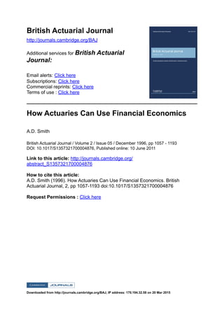
![B.A.J.2,V, 1057-1193(1996)
HOW ACTUARIES CAN USE FINANCIAL ECONOMICS
B Y A . D . SMITH, B.A.
[Presented to the Institute of Actuaries, 25 March 1996]
ABSTRACT
There has recently been some debate about the usefulness of financial economics to the actuarial
profession. The consensus appears to be that the techniques are potentially valuable, but the published
material is not quite 'oven ready'. Some development work is required before the material can be
applied.
The author has carried out much of the necessary development work on behalf of various clients
over the last few years. On some occasions the results have conflicted with more conventional
actuarial methods. The main aim of the paper is to bring the new techniques into the public domain
so that they can be properly discussed by the profession, and adopted more widely if appropriate.
The paper contains a number of worked examples using techniques developed by financial
economists. The author has listed the computer code which generated the examples and deposited
copies on the Internet, so that others can explore the issues with a minimal development overhead.
KEYWORDS
Financial Economics; Stochastic Models; Asset-Liability Studies; Dynamic Optimisation;
Equilibrium; Arbitrage; Risk-Neutral Law
1. INTRODUCTION
1.1 Financial economics is the application of economic theory to financial
markets. Its use in actuarial work continues to be controversial. At one extreme,
I have seen models applied uncritically in apparently blind faith, while at the
other extreme, some actuaries have claimed that financial economics is part of a
conspiracy to displace traditional methods with unsound practices (see, for
example, Clarkson in the discussion of Bride & Lomax, 1994).
1.2 Financial economics has produced several specific models which have
come into widespread use within the financial community. Examples include the
capital asset pricing model, or CAPM, as derived by Sharpe (1964) and the Black
& Scholes (1973) formula for option pricing. There are also a number of
established models describing the term structure of interest rates and the pricing
of associated derivatives, such as Ho & Lee (1986), Hull & White (1990) and
Black, Derman & Toy (1990). Several actuarial papers have been published
applying such models. Examples include Wilkie (1987) who applies option
pricing to bonus policy, or Mehta (1992) who, inter alia, demonstrates the use of
the CAPM to derive discount rates for calculating appraisal values.
1.3 It is not the purpose of this paper to review established models such as
the CAPM or the Black-Scholes formula. Instead, I will examine some underlying
1057](data:image/gif;base64,R0lGODlhAQABAIAAAAAAAP///yH5BAEAAAAALAAAAAABAAEAAAIBRAA7)