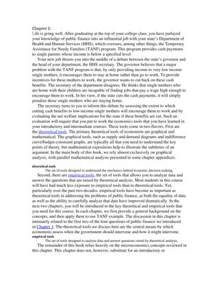
SlideShare une entreprise Scribd logo
1  sur  31
Télécharger pour lire hors ligne
Chapter 2:
Life is going well. After graduating at the top of your college class, you have parlayed 
your knowledge of public finance into an influential job with your state’s Department of 
Health and Human Services (HHS), which oversees, among other things, the Temporary 
Assistance for Needy Families (TANF) program. This program provides cash payments 
to single parents whose income is below a specified level.
Your new job thrusts you into the middle of a debate between the state’s governor and 
the head of your department, the HHS secretary. The governor believes that a major 
problem with the TANF program is that, by only providing income to very low income 
single mothers, it encourages them to stay at home rather than go to work. To provide 
incentives for these mothers to work, the governor wants to cut back on these cash 
benefits. The secretary of the department disagrees. He thinks that single mothers who 
are home with their children are incapable of finding jobs that pay a wage high enough to
encourage them to work. In his view, if the state cuts the cash payments, it will simply 
penalize those single mothers who are staying home.
The secretary turns to you to inform this debate by assessing the extent to which 
cutting cash benefits to low­income single mothers will encourage them to work and by 
evaluating the net welfare implications for the state if these benefits are cut. Such an 
evaluation will require that you put to work the economics tools that you have learned in 
your introductory and intermediate courses. These tools come in two flavors. First are 
the theoretical tools. The primary theoretical tools of economists are graphical and 
mathematical. The graphical tools, such as supply and demand diagrams and indifference 
curve/budget constraint graphs, are typically all that you need to understand the key 
points of theory, but mathematical expositions help to illustrate the subtleties of an 
argument. In the main body of this book, we rely almost exclusively on graphical 
analysis, with parallel mathematical analysis presented in some chapter appendices.
theoretical tools
The set of tools designed to understand the mechanics behind economic decision making.
Second, there are empirical tools, the set of tools that allows you to analyze data and 
answer the questions that are raised by theoretical analysis. Most students in this course 
will have had much less exposure to empirical tools than to theoretical tools. Yet, 
particularly over the past two decades, empirical tools have become as important as 
theoretical tools in addressing the problems of public finance, as both the equality of data 
as well as the ability to carefully analyze that data have improved dramatically. In the 
next two chapters, you will be introduced to the key theoretical and empirical tools that 
you need for this course. In each chapter, we first provide a general background on the 
concepts, and then apply them to our TANF example. The discussion in this chapter is 
intimately related to the first two of the four questions of public finance we introduced 
in Chapter 1. The theoretical tools we discuss here are the central means by which 
economists assess when the government should intervene and how it might intervene.
empirical tools
The set of tools designed to analyze data and answer questions raised by theoretical analysis.
The remainder of this book relies heavily on the microeconomics concepts reviewed in
this chapter. This chapter does not, however, substitute for an introductory or 
intermediate microeconomics course. The goal here is to refresh your understanding of 
the important concepts that you need to undertake theoretical public finance, not to teach 
them to you for the first time. If the material in this chapter is very unfamiliar, you may 
want to supplement this text with a more detailed microeconomics text.1
Constrained Utility Maximization
The core of theoretical analysis in public finance is the assumption that individuals have well­
defined utility functions, a mathematical mapping of individual choices over goods into their level of well­
being. Economists assume that individuals then undertake constrained utility maximization, maximizing 
their well­being (utility) subject to their available resources. Armed with this assumption, economists 
proceed to develop models—mathematical or graphical representations of reality—to show how 
constrained utility maximization leads people to make the decisions that they make every day. These 
models have two key components: the individual’s preferences over all possible choices of goods and 
her budget constraint, the amount of resources with which she can finance her purchases. The strategy of 
economic modelers is then to ask: Given a budget constraint, what bundle of goods makes a consumer best 
off?
utility function
A mathematical function representing an individual’s set of preferences, which translates her well-
being from different consumption bundles into units that can be compared in order to determine
choice.
constrained utility maximization
The process of maximizing the well-being (utility) of an individual, subject to her resources
(budget constraint).
models
Mathematical or graphical representations of reality.
We can illustrate how consumers are presumed to make choices in four steps. First, we discuss how to 
model preferences graphically. Then, we show how to take this graphical model of preferences and 
represent it mathematically with a utility function. Third, we model the budget constraints that individuals 
face. Finally, we show how individuals maximize their utility (make themselves as well off as possible) 
given their budget constraints.
Preferences and Indifference Curves
In modeling people’s preferences, we are not yet imposing any budget constraints; we are
simply asking what people prefer, ignoring what they can afford. Later, we impose 
budget constraints to round out the model.
Much of the power of the preferences models we use in this course derives from one 
simple assumption: non­satiation, or “more is better.” Economists assume that more of a 
good is always better than less. This does not mean that you are equally happy with the 
tenth pizza as you are with the first; indeed, as we learn later, your happiness increases 
less with each additional unit of a good you consume. Non­satiation simply implies that 
having that tenth pizza is better than not having it.
Armed with this central assumption, we can move on to graphically represent a 
consumer’s preferences across different bundles of goods. Suppose, for example, 
that Figure 2­1 represents Andrea’s preferences between two goods, cakes (with 
quantity QC) and movies (with quantity QM). Consider three bundles:
Bundle A: 2 cakes and 1 movie
Bundle B: 1 cake and 2 movies
Bundle C: 2 cakes and 2 movies
Let’s assume, for now, that Andrea is indifferent between bundles A and B, but that 
she prefers C to either; she clearly prefers C because of the assumption that more is 
better. Given this assumption, we can map her preferences across the goods. We do so 
using an indifference curve, a curve that shows all combinations of consumption that give
the individual the same amount of utility (and so among which the individual is 
indifferent). In this case, Andrea gets the same utility from bundles A and B, so they lie 
on the same indifference curve. Because she gets a higher level of utility from consuming
bundle C instead of either A or B, bundle C is on a higher indifference curve.
indifference curve
A graphical representation of all bundles of goods that make an individual equally well off.
Because these bundles have equal utility, an individual is indifferent as to which bundle she
consumes.
Indifference curves have two essential properties, both of which follow naturally from 
the more­is­better assumption:
1. Consumers prefer higher indifference curves. Individuals prefer to 
consume bundles that are located on indifference curves that are farther out 
from the origin because they represent bundles that have more of, for example, 
both cakes and movies.
2. Indifference curves always slope downward. Indifference curves cannot 
slope upward because that would imply that, in this instance, Andrea is 
indifferent between a given bundle and another bundle that has more of both 
cakes and movies, which violates the more­is­better assumption.
A great example of indifference curve analysis is job choice. Suppose that Sam 
graduates and is considering two attributes as he searches across jobs: the starting salary 
and the location of the job. Sam prefers both a higher salary and a location with a higher 
average temperature because he hates cold weather. We can represent Sam’s preferences 
using Figure 2­2, which shows the trade­off between salary and location (temperature). 
Sam has three job choices:
Figure 2­2Indifference Curve Analysis 
of Job Choice • In choosing a job, Sam trades off the two things he cares about, salary and location (average temperature). 
On IC1, he is indifferent between a job in Minneapolis, with a high salary and a low average temperature, and one in Phoenix, with 
a lower salary and a higher average temperature. However, as indicated by its position on IC2, he prefers a job in Washington, 
D.C., with an average salary and an average temperature.
Bundle A: Starting salary of $30,000 in Phoenix, AZ (hot!)
Bundle B: Starting salary of $50,000 in Minneapolis, MN (cold!)
Bundle C: Starting salary of $40,000 in Washington, D.C. (moderate)
Given Sam’s preferences, it may be that he is indifferent between bundles A and B—that is, the higher 
starting salary in Minneapolis is enough to compensate him for the much colder weather. But he may 
prefer C to either: the salary in Washington is higher than in Phoenix, and the weather is much warmer than
in Minneapolis. Compromising on salary and location leaves Sam better off than choosing an extreme of 
one or the other in this example.
Utility Mapping of Preferences
Underlying the derivation of indifference curves is the notion that each individual has a well­defined utility
function. A utility function is a mathematical representation U = f (X1, X2, X3, . . .), where X1, X2, X3, and so 
on are the goods consumed by the individual and f is some mathematical function that describes how the 
consumption of those goods translates to utility. This mathematical representation allows us to compare the
well­being associated with different levels of goods consumption.
For example, suppose that Andrea’s utility function for cakes and movies is U=√QC×QM .
With this function, she would be indifferent between 4 cakes and 1 movie, 2 cakes and 2 movies, and 1 
cake and 4 movies because each of these bundles would deliver a utility level of 2. But she would prefer 3 
cakes and 3 movies to any of these bundles because this would give her a utility level of 3.
Marginal Utility
The key concept for understanding consumer preferences is marginal utility, or the 
additional increment to utility from consuming an additional unit of a good. This 
described utility function exhibits the important principle of diminishing marginal 
utility: the consumption of each additional unit of a good makes an individual less happy 
than the consumption of the previous unit. To see this, Figure 2­3 graphs the marginal 
utility, the increment to utility from each additional movie seen, holding the number of 
cakes constant at 2. When Andrea moves from seeing 0 movies to seeing 1 movie, her 
utility rises from 0 to √ 2 =1.41.  Thus, the marginal utility of that first movie is 
1.41. When she moves from seeing one movie to seeing a second movie, her utility rises 
to √4=2.  The consumption of the second movie has increased utility by only 0.59, 
a much smaller increment than 1.41. When she sees a third movie, her utility rises to 
only √6=2.45,  for an even smaller increment of 0.45. With each additional movie
consumed, utility increases, but by ever smaller amounts.
Figure 2­3Diminishing Marginal 
Utility • Holding the number of cakes constant at 2, with a utility function of U=√ QC×QM,  each additional movie 
consumed raises utility by less and less.
marginal utility
The additional increment to utility obtained by consuming an additional unit
of a good.
Why does diminishing marginal utility make sense? Consider the example of movies. There is almost 
always one particular movie that you want to see the most, then one which is next best, and so on. So you 
get the highest marginal utility from the first movie you see, less from the next, and so on. Similarly, think 
about slices of pizza: when you are hungry, you get the highest increment to your utility from the first slice;
by the fourth or fifth slice, you get much less utility per slice.
Marginal Rate of Substitution
Armed with the concept of marginal utility, we can now describe more carefully exactly what indifference 
curves tell us about choices. The slope of the indifference curve is the rate at which a consumer is willing to
trade off the good on the vertical axis for the good on the horizontal axis. This rate of trade­off is called 
the marginal rate of substitution (MRS). In this example, the MRS is the rate at which Andrea is willing to 
trade cakes for movies. As she moves along the indifference curve from more cakes and fewer movies to 
fewer cakes and more movies, she is trading cakes for movies. The slope of the curve tells Andrea the rate 
of trade that leaves her indifferent between various bundles of the two goods.
marginal rate of substitution (MRS)
The rate at which a consumer is willing to trade one good for another.
The MRS equals the slope of the indifference curve, the rate at which the
consumer will trade the good on the vertical axis for the good on the
horizontal axis.
For the utility functions we use in this book, such as Andrea’s, the MRS is diminishing. We can see this 
by graphing the indifference curves that arise from the assumed utility function U=√QC×QM.  
As Figure 2­4 shows, Andrea is indifferent between 1 movie and 4 cakes, 2 movies and 2 cakes, and 4 
movies and 1 cake. Along any segment of this indifference curve, we can define an MRS. For example, 
moving from 4 CDs and 1 movie to 2 cakes and 2 movies, the MRS is −2; she is willing to give up 2 cakes 
to get 1 additional movie. Moving from 2 cakes and 2 movies to 1 cake and 4 movies, however, the MRS is 
−½ she is willing to give up only 1 cake to get 2 additional movies.
Figure 2­4Marginal Rates of Substitution • With a utility function of U=√ QC×QM,  MRS diminishes as the 
number of movies consumed increases. At 4 cakes and 1 movie, Andrea is willing to trade 2 cakes to get 1 movie (MRS =−2). At 2
cakes and 2 movies, Andrea is willing to trade 1 cake to get 2 movies (MRS = −½).
The slope of the indifference curve changes because of diminishing MRS. When Andrea is seeing only 
1 movie, getting to see her second­choice movie is worth a lot to her, so she is willing to forgo 2 cakes for 
that movie. But, having seen her second­choice movie, getting to see her third­ and fourth­choice movies 
isn’t worth so much, so she will only forgo 1 cake to see them. Thus, the principle of diminishing MRS is 
based on the notion that as Andrea has more and more of good A, she is less and less willing to give up 
some of good B to get additional units of A.
Because indifference curves are graphical representations of the utility function, there is a direct 
relationship between the MRS and utility: the MRS is the ratio of the marginal utility for movies to the 
marginal utility for cakes:
MRS = –MUM/MUC
That is, the MRS shows how the relative marginal utilities evolve over the indifference curve: as Andrea 
moves down the curve, the MU of cakes rises and that of movies falls. Remember that higher quantity 
implies lower marginal utility, by the principle of diminishing marginal utility. As Andrea moves down the 
indifference curve, getting more movies and fewer cakes, the marginal utility of cakes rises, and the 
marginal utility of movies falls, lowering the MRS.
Budget Constraints
If the fundamental principle of consumer choice is that more is better, what keeps folks from simply 
bingeing on everything? What stops them is their limited resources, or their budget constraint, a 
mathematical representation of the combination of goods they can afford to buy given their incomes. For 
the purposes of this discussion, we make the simplifying assumption that consumers spend all their income;
there is no savings. In Chapter 22, we discuss the implications of a more realistic model where individuals 
can save and borrow, but for now we will assume that all income is spent in the period in which it is 
received. Moreover, for the purposes of this example, let’s assume that Andrea spends her entire income on
CDs and movies.
budget constraint
A mathematical representation of all the combinations of goods an individual
can afford to buy if she spends her entire income.
Given these assumptions, Andrea’s budget constraint is represented mathematically by Y = 
PCQC + PMQM, where Y is her income, PC and PM are the prices of cakes and movies, and QC and QM are the 
quantities of cakes and movies she buys. That is, this expression says that her expenditures on cakes and on
movies add up to be her total income.
Graphically, the budget constraint is represented by the line AB in Figure 2­5. The horizontal intercept 
is the number of movies that Andrea can buy if she purchases no cakes, the vertical intercept is the number 
of cakes she can buy if she goes to no movies, and the slope of the budget constraint is the rate at which the
market allows her to trade off cakes for movies. This rate is the negative of the price ratio PM/PC: each extra 
movie that she buys, holding income constant, must lower the number of cakes that she can buy by PM/PC.
Figure 2­5Budget Constraint • With an income, Y, of $96, a price of $16 per cake, and a price of $8 per movie, Andrea 
can trade off 1 cake for 2 movies, up to a total of either 6 cakes or 12 movies. The slope of the budget constraint is therefore 2 
1.2, indicating the ratio of movie­to­cakeprices.
Figure 2­5 illustrates the budget constraint for the case when Y = $96, PC = $16, and PM = $8. At this 
income and these prices, Andrea can purchase 12 movies or 6 cakes, and each cake she buys means that she
can buy fewer movies. The slope of the budget constraint is the rate at which she can trade cakes for 
movies in the marketplace, PM/PC = –8
/16 = –½.
Quick Hint Our discussion thus far has been couched in terms of “trading cakes for movies” and 
vice versa. In reality, however, we don’t directly trade one good for another; instead, we trade in a 
market economy, in which cakes and movies are purchased using dollars. The reason we say 
“trading cakes for movies” is because of the central economics concept of opportunity cost, which 
says that the cost of any purchase is the next best alternative use of that money. Thus, given a fixed
budget, when a person buys a cake, she forgoes the opportunity to see two movies. In essence, 
she is trading the cake for two movies, even though, in reality, she accomplishes the trade using 
money rather than the goods themselves. When a person’s budget is fixed, if she buys one thing, 
she is, by definition, reducing the money she has to spend on other things. Indirectly, this purchase 
has the same effect as a direct good­for­good trade.
opportunity cost
The cost of any purchase is the next best alternative use of that money, or the
forgone opportunity.
Putting It All Together: Constrained Choice
Armed with the notions of utility functions and budget constraints, we can now ask: What is the utility­
maximizing bundle that consumers can afford? That is, what bundle of goods makes consumers best off, 
given their limited resources?
The answer to this question is shown in Figure 2­6. This figure puts together the indifference curves 
corresponding to the utility function U=√QC×QM,  shown in Figure 2­4 with the budget 
constraint shown in Figure 2­5. In this framework, we can rephrase our question: What is the highest 
indifference curve that an individual can reach given a budget constraint? The answer is the indifference 
curve, IC2, that is tangent to the budget constraint: this is the farthest­out indifference curve that is 
attainable, given Andrea’s income and market prices. In this example, Andrea makes herself as well off as 
possible by choosing to consume 6 movies and 3 cakes (point A). That combination of goods maximizes 
Andrea’s utility, given her available resources and market prices.
Figure 2­6Constrained Optimization • Given a utility function of U=√ QC×QM,  an income of $96, and prices of 
cakes and movies of $16 and $8, respectively, Andrea’s optimal choice is 3 cakes and 6 movies (point A). This represents the 
highest indifference curve she can reach, given her resources and market prices. She can also afford points such as B and C, but 
they leave her on a lower indifference curve (IC1 instead of IC2).
The key to understanding this outcome is the marginal decision Andrea makes to consume the next 
movie. The benefit to her of consuming another movie is the marginal rate of substitution,the rate at which 
she is willing to trade cakes for movies. The cost to her of making this trade is the price ratio, the rate at 
which the market allows her to trade cakes for movies. Thus, the optimal choice is the one at which:
MRS = −MUM/MUC = −PM/PC
At the optimum, the ratio of marginal utilities equals the ratio of prices. The rate at which Andrea is willing
to trade off one good for the other is equal to the rate at which the market will let her carry out that trade.
One way to demonstrate that this is the optimal choice is to show that she is worse off with any other 
choice. Consider point B in Figure 2­6. At that point, the slope of the indifference curve IC1is higher than 
the slope of the budget constraint; that is, the MRS is greater than the price ratio. This means that Andrea’s 
marginal utility of movies, relative to cakes, is higher than the ratio of the price of movies to the price of 
cakes. Because the MRS is the rate at which Andrea is willing to trade cakes for movies, and the price ratio 
is the rate that the market is charging for such a trade, Andrea is willing to give up more cakes for movies 
than the market requires. She can make herself better off by reducing her cake purchases and increasing her
movie purchases, as happens when she moves from B to A.
Now consider point C in Figure 2­6. At this point, the slope of the indifference curve IC1 is less than the
slope of the budget constraint; that is, the MRS is lower than the price ratio. Relative to point B, Andrea 
now cares much less about movies and more about cakes because she is now consuming more movies and 
fewer cakes, and marginal utility diminishes. At point C, in fact, she is willing to give up fewer cakes for 
movies than the market requires. So she can make herself better off by increasing her cake purchases and 
reducing her movie purchases, as happens when she moves from C to A. Whenever a consumer is at a point
where the indifference curve and the budget constraint are not tangent, she can make herself better off by 
moving to a point of tangency.
Quick Hint Marginal analysis, the consideration of the costs and benefits of an additional unit of 
consumption or production, is a central concept in modeling an individual’s choice of goods and a 
firm’s production decision. All optimization exercises in economics are like climbing a hill on a very 
foggy day. At any given point, you don’t know yet whether you are at the top, but you do know if you
are heading up or heading down. If you are heading up, then you must not yet be at the top; but if 
you are heading down, then you must have passed the top.
It is the same when you are maximizing your utility (or your firm’s profits). Consider the 
mountain as your decision about how many movies to buy and the top as the optimal number of 
movies given your preferences and budget constraint. Starting from any number of cakes and 
movies, you consider whether the next movie has a benefit (MRS) greater than its cost (price ratio). 
If the benefit exceeds the cost of that next movie, then the next step is upward, and you buy the 
movie and continue up the optimization mountain. If the benefit is below the cost, then the next step 
is downward, and you realize that you need to go backward (buy fewer movies) to get back to the 
top. Only when the benefit equals the cost of the next unit do you realize you are at the top of the 
mountain.
The Effects of Price Changes: Substitution and Income Effects
The key result from the constrained choice analysis is that MUM/MUC = PM/PC: Andrea consumes movies 
and cakes until the ratio of the marginal utility of movies to cakes equals the ratio of their prices. This 
result implies that when the relative price of a good, such as movies in our example, rises 
(i.e., PM/PC rises), then the relative quantity of that good demanded falls. This is because, for the equality 
previously described to hold, when PM/PC rises, then MUM/MUC must also rise. For MUM/MUC to rise, the 
quantity of movies relative to cakes must fall (because the marginal utility of any good falls as the quantity 
consumed of that good rises).
This point is illustrated graphically in Figure 2­7. We have already shown that, with an income of $96, 
and prices of $16 for cakes and $8 for movies, Andrea chooses 6 movies and 3 cakes at point A, the point at
which BC1 and IC1 are tangent. If the price of movies were to rise to $16, for example, the budget constraint
would become steeper; it rotates inward from BC1 to BC2.
Figure 2­7Substitution 
and Income Effects • When the price of movies increases, it has two effects. First, holding utility constant, there is a substitution 
effect, which causes Andrea to demand fewer movies because they are relatively more expensive (moving from point A to 
point B). Second, holding relative prices constant, there is an income effect, which causes her to demand fewer movies because 
she is poorer (moving from point B to point C).
Because the price of cakes hasn’t changed, Andrea can still buy 6 cakes with her $96 
income (the vertical intercept of the budget constraint), but because the price of movies 
has risen to $16, she can only now buy 6 ($96/$16) movies (the horizontal intercept). The
slope of the budget constraint rises from −½ to −1, as illustrated by BC2.
With a steeper budget constraint, Andrea can no longer afford to buy the combination 
at point A. The optimal combination becomes point C, the point at which BC2 is tangent 
to a lower indifference curve, IC2. At this point, Andrea can buy 3 cakes, but she can now
only buy 3 movies, instead of the 6 she could buy at point A. The quantity of movies she 
demands has fallen because their price has gone up. She is also now worse off: her 
budget set, or the set of possible choices she can make given her income, has been 
restricted (because the budget constraint moved inward from BC1 to BC2). The quantity of
cakes she demands has remained constant, but this is only because of the assumed 
mathematical form of the utility function; in general, the number of cakes she demands 
would fall as well.
Income and Substitution Effects
Imagine that the government could somehow insulate Andrea from the utility she loses when prices rise; 
that is, suppose the government was somehow able to compensate her enough that she could stay on 
the same indifference curve (IC1, in our example), even with the new set of prices. Would this mean that the
price change will have no effect on her choices? No, it wouldn’t, because she would still like to choose a 
different bundle of cakes and movies at this new set of prices.
Figure 2­7 also illustrates this point. Despite this price change, the government can hold Andrea’s utility
constant at these new prices by giving her a budget constraint BCg, which is parallel to BC2 but tangent to 
the same indifference curve IC1 that corresponds to her original choice. Graphically, the budget constraint 
has steepened, but Andrea is on the same indifference curve (the same level of utility). Andrea chooses the 
bundle represented by point B: because movies are relatively more expensive, she chooses to consume 
fewer movies (4.24) and more cakes (4.24). This effect of a price change is called the substitution effect: 
holding utility constant, a relative rise in the price of a good will always cause a consumer to choose less of
that good.
substitution effect
Holding utility constant, a relative rise in the price of a good will always cause
an individual to choose less of that good.
income effect
A rise in the price of a good will typically cause an individual to choose less of
all goods because her income can purchase less than before.
normal goods
Goods for which demand increases as income rises.
inferior goods
Goods for which demand falls as income rises.
In the real world, when prices rise, there is no government agency to hold utility constant. This price 
rise therefore leads to a second effect on demand: Andrea is now effectively poorer because she has to pay 
higher prices for movies. She is not poorer in an income sense (her income remains at $96), but she is 
poorer in a real sense because her $96 can buy fewer goods (in particular, fewer movies). This is 
the income effect of a price change: a rise in any price will make the consumer effectively poorer, causing 
her to choose less of all goods.2
 The quantity demanded falls because Andrea can buy fewer goods with her 
income.
We can measure this income effect by the change from the government­supported budget 
constraint BCg to the new budget constraint BC2. This change represents the restriction in Andrea’s 
opportunity set at the new prices. Because she is poorer, she chooses fewer of all goods, including both 
movies and cakes, at point C. In this case, the income effect reinforces the substitution effect for movies: 
both cause the quantity of movies she demands to fall.3
 To sum up, when the price of one good increases 
relative to another, you choose less of that good for two reasons: because it is relatively more expensive 
(the substitution effect) and because you are effectively poorer (the income effect).
Putting the Tools to Work: TANF and Labor Supply Among Single Mothers
In your new position with the state government, you have now reviewed the theoretical 
concepts necessary to address the concerns of the secretary and the governor. Having 
reviewed these theoretical concepts, let’s turn to the question posed at the start of the 
chapter: Will reducing TANF benefits increase the labor supply of single mothers? To 
answer this question, we can apply the tools of utility maximization to the analysis of the 
labor supply decision.
The TANF program was created in 1996 by a major overhaul of the cash 
welfare system in the United States. The cash welfare system distributes money from 
taxpayers to low­income families (as described in much more detail in Chapter 17). 
TANF provides a monthly support check to families with incomes below a threshold 
level that is set by each state. In the state of New Jersey, for example, a single mother 
with two children and no other source of income will receive a monthly check for 
$424.4
 These checks are largely targeted to single­female­headed households with 
children because these families are viewed as having the worst prospects for making a 
living on their own.
Suppose that Joelle is a single mother who spends all of her earnings and TANF 
benefits on food for herself and her children. By working more hours, she can earn more 
money for food, but there is a cost to work: she has less time at home with her children 
(or less time to spend on her own leisure). Suppose that she would prefer time at home to 
time at work; that is, suppose that leisure is a normal good. With these preferences, more 
work makes Joelle worse off, but it allows her to buy more food.
How does Joelle decide on the optimal amount of labor to supply? To answer this 
question, we return to the utility maximization framework, but with one twist relative to 
the decision to purchase cakes and movies. In that case, we were considering two goods. 
Now, the single mother is considering one good (food consumption) and one “bad” 
(labor, as we assume she would rather be at home than at work). The trick to modeling 
this decision is to model the demand for leisure,the good that is the counterpart of labor. 
That way, we can model the trade­off between two goods using our existing tools and 
then compute the amount of labor supplied as total work hours minus hours of leisure.
Identifying the Budget Constraint
Suppose that Joelle can work up to 2,000 hours per year at a wage of $10 per hour, that she has no other 
source of income, and that there is not yet a TANF program in place. By working one less hour in a year, 
Joelle will lower her consumption by $10 and increase her leisure time by one hour. Thus, the “price” of 
one hour of leisure time is the hourly wage rate. This fact follows from the principle of opportunity cost: 
when Joelle opts to take an hour of leisure, her next best alternative activity is to work. Thus, the price of 
the hour of leisure is $10, the forgone wage she could have earned if working.
The price of food consumption is given directly by the market; let’s say that it is $1 per unit of food. 
This means that Joelle faces a trade­off: each hour of work brings her 10 units of food, and each hour off 
from work (leisure) costs her 10 units of food. If Joelle can work up to 2,000 hours per year, we can now 
identify her budget constraint as line ABC in Figure 2­8: she can consume a maximum of $20,000 of food 
per year, a maximum of 2,000 hours of leisure per year, or any combination in between. The slope of the 
budget constraint is the negative of the ratio of the price of leisure ($10) to the price of consumption ($1), 
−10.
Figure 2­8The Consumption–
Leisure Trade­off • Joelle has a choice of taking more leisure and consuming less or taking less leisure (working harder) and 
consuming more. If she takes no leisure, she can have consumption of $20,000 per year; but if she takes 2,000 hours of leisure, 
her consumption falls to 0. This is represented by the budget constraint with a slope of −10, the relative price of leisure in terms of 
food consumption.
The Effect of TANF on the Budget Constraint
Now, let’s introduce a TANF program and illustrate what this does to the budget 
constraint. Programs such as TANF typically have two key features. The first is a benefit 
guarantee, or the baseline amount of money to which recipients are entitled when they 
enroll in the program. The second is a benefit reduction rate, the rate at which the 
baseline amount is reduced if recipients have other income. For example, a benefit 
reduction rate of 100% implies that TANF recipients are entitled to the benefit guarantee 
if they have no other income, but that they lose a dollar of the benefit guarantee for each 
dollar of other income they earn. A benefit reduction rate of only 50% implies that TANF
recipients once again get the full benefit guarantee if they have no other income, but that 
they lose $0.50 of the benefit guarantee for each $1 they earn. The benefit reduction rate 
is, in effect, an implicit tax rate; it is the rate at which TANF benefits are reduced when 
recipients earn other income.
We can now add the TANF program to the budget constraint in panel (a) of Figure 2­
9. Let’s assume the TANF program we’re considering has a benefit guarantee of $5,000 
and a benefit reduction rate of 50%. The original budget constraint is the line ABC. If 
Joelle chooses 1,000 or fewer hours of leisure, earning $10,000 to $20,000, the budget 
constraint does not change, remaining as the segment AB. This is because, with a benefit 
guarantee of $5,000 and a benefit reduction rate of 50%, once she earns $10,000 
($5,000/0.5), she is no longer eligible for TANF, so it doesn’t affect her budget 
constraint.
The Budget Constraint with TANF
• Joelle’s original budget constraint is ABC. With a TANF guarantee of $5,000 and a benefit reduction rate of
50% in panel (a), the budget constraint becomes ABD. Once she has taken more than 1,000 hours of 
leisure, the budget constraint flattens, and she now can enjoy $5,000 of consumption even with 2,000 hours 
of leisure at point D. When the guarantee falls to $3,000 in panel (b), the budget constraint (AEF) doesn’t 
flatten until she tak
If Joelle chooses to take more than 1,000 hours of leisure, however, the budget 
constraint is now flatter. Previously, the price of leisure was $10 per hour because that 
was the forgone wage. With the 50% benefit reduction rate, however, if Joelle works 
another hour, she earns $10 in wages but loses $5 in TANF benefits. Under these 
conditions, the net return to working another hour is now only $5, so the price of leisure 
falls to $5 per hour. The budget constraint is therefore flatter, with a slope of only −5 
rather than −10, because in the range where TANF is available, there is a lower relative 
price of leisure. Point D marks the end of the new budget constraint and provides a new 
option for Joelle: she can have 2,000 hours of leisure and $5,000 in food consumption 
because of the $5,000 TANF benefit guarantee. Without TANF, if she had chosen to 
consume 2,000 hours of leisure, she wouldn’t have been working at all, and her family 
would have had no food (point C).
Effects of Changes in Benefit Guarantee
Suppose that your state is considering reducing the income guarantee under TANF from $5,000 to $3,000. 
The effect of this change on the budget constraint is illustrated in panel (b) of Figure 2­9. If Joelle now 
chooses to take fewer than 1,400 hours of leisure, earning $6,000 to $20,000, the budget constraint does not
change, remaining as the segment AE. This is because, with the lower benefit guarantee of $3,000 and a 
benefit reduction rate of 50%, she is now no longer eligible for TANF once she earns $6,000. If she takes 
more than 1,400 hours of leisure, the budget constraint once again flattens: because she earns $10 in wages 
but loses $5 in TANF benefits for each hour of work in this range, the slope of the budget constraint along 
the segment EF (the net return to an hour of work) is −5. Point F marks the end of the new budget 
constraint, where Joelle can have 2,000 hours of leisure and $3,000 in food consumption because of the 
$3,000 TANF benefit guarantee. How will single mothers react to this policy change?
In answering this question, it is important to return to the concepts of income and substitution 
effects introduced earlier. Suppose, for example, that Joelle earned less than $6,000 before this benefit 
change. In that case, there is no substitution effect associated with the policy change from a $5,000 benefit 
guarantee to a $3,000 benefit guarantee. There is no change in the relative price of leisure, which remains at
$5 per hour, so the slope of the budget constraint doesn’t change. Whether Joelle gets a $5,000 or a $3,000 
check from the government has no impact on the return from working an additional hour ($5 on net), so the
price of leisure is unchanged. With relative prices of food and leisure unchanged, there is no desire for 
substitution across the goods.
There is, however, a clear income effect for Joelle. When the TANF guarantee is reduced, she is poorer.
Poorer individuals will reduce their consumption of all normal goods, including leisure. Taking less leisure 
means working more. In other words, because there is less money available to finance consumption, 
women will have to work harder. Thus, on net, there is a reduction in leisure from the income effect of 
reducing the TANF guarantee.
Suppose, instead, that Joelle earned between $6,000 and $10,000 before the benefit change. Once again,
this benefit change reduces her income, which will cause her to choose less leisure (and more labor). There 
is also, however, a change in the price of leisure. In this range of earnings, before the benefits change, an 
hour of work netted Joelle only $5 per hour, due to the reduction in TANF benefits from additional 
earnings. Now, because she is no longer eligible for TANF in this income range, an hour of work nets her 
$10. This relative increase in the price of leisure (taking leisure used to cost $5 but now costs $10 in 
forgone earnings) will lead to a substitution effect toward less leisure. Thus, in this range, the income and 
substitution effects work together to reduce leisure.
How Large Will the Labor Supply Response Be?
This example illustrates the power of economic theory. The constrained maximization model implies that a 
reduction in the benefit guarantee will lead to less leisure and, therefore, more work among single mothers. 
The model does not say, however, how sizeable this response will be. This depends on how much Joelle 
earned before the benefit change, and the size of the income and substitution effects on her leisure/labor 
decision.
To illustrate the different possible magnitudes of the response, Figures 2­10 and 2­11 show two 
different cases. In both cases, we consider utility functions for consumption and leisure, where the utility 
derived from each is proportional to its natural logarithm (ln). This is a convenient form for utility 
functions that shares most of the properties of the square root utility function we used for cakes and 
movies, most notably diminishing marginal utility. As noted earlier, the square root and log forms are just 
two of many possible forms for utility.
Utility Maximization for Sarah 
• When the TANF guarantee is $5,000, the optimal choice for Sarah is to take 1,910 hours of leisure and 
consume $5,450 (at point A). When the guarantee falls to $3,000, she reduces her leisure to 1,655 hours, 
and her consumption falls to $4,725 (at point B).
Figure 2­11Utility Maximization 
for Naomi • Because Naomi values leisure more highly relative to consumption than Sarah in Figure 2­10, she chooses 2,000 
hours of leisure regardless of the TANF guarantee. The reduction in guarantee therefore lowers Naomi’s consumption from 
$5,000 (at point A) to $3,000 (at point B).
The first mother, Sarah, has a utility function of the form U = 100 − ln(C) + 175 − 
ln(L), where C is consumption, L is leisure, and ln is the natural logarithmic function. 
Sarah values both consumption and leisure, but she values leisure somewhat more. Figure
2­10 shows her indifference curves and budget constraint. When the guarantee is $5,000, 
Sarah chooses to consume 1,910 hours of leisure and work 90 hours per year 
(point A, where her indifference curve is tangent to the budget constraint with a $5,000 
guarantee). At that level of labor supply, her wage earnings are $900. Because her TANF 
guarantee is reduced by $0.50 for each $1 of earnings, however, her total income is the 
$900 in earnings plus a net TANF benefit of $5,000 − 0.5 × $900 = $4,550. So her total 
consumption expenditures are $900 + $4,550 = $5,450. (The mathematics of this example
is shown in the appendix to this chapter.)
When the TANF guarantee is reduced to $3,000, Sarah chooses to reduce her leisure 
because she is now poorer (the income effect), moving to point B on the new budget 
constraint. At that point, she takes only 1,655 hours of leisure per year, works 345 hours, 
and earns $3,450. For this mother, the governor is right; the reduction in TANF guarantee
has raised her labor supply from 90 hours to 345 hours. Note that because Sarah’s TANF 
benefits are reduced by half her earnings, her TANF benefits are now $3,000 − 0.5 − 
$3,450 = $1,275. Thus, her total budget is $4,725; her consumption has fallen by $725 
from the days of the higher TANF guarantee ($5,450 – $4,725 = $725). Her consumption
has not fallen by the full $2,000 cut in the guarantee because she has compensated for the
guarantee reduction by working harder.
Figure 2­11 illustrates the case of a different single mother, Naomi, with a utility 
function U = 75 × ln(C) + 300 × ln(L). Naomi puts a much larger weight on leisure 
relative to consumption, when compared to Sarah. (Her indifference curves are steeper, 
indicating that a larger increase in consumption is required to compensate for any 
reduction in leisure.) For Naomi, the optimal choice when the TANF guarantee is $5,000 
is to not work at all; she consumes 2,000 hours of leisure and $5,000 of food (point A). 
When the guarantee is reduced to $3,000, this mother continues not to work and just lets 
her consumption fall to $3,000. That is, she cares so much more about leisure than about 
consumption that she won’t supplement her TANF guarantee with earnings even at the 
lower guarantee level. For this mother, the secretary is right; the reduction in TANF 
guarantee has had no effect on labor supply, it has simply cut her level of food 
consumption.
Thus, theory alone cannot tell you whether this policy change will increase labor 
supply or by how much. Theoretically, labor supply could rise, but it might not. To move 
beyond this uncertainty, you will have to analyze available data on single mother labor 
supply, and the next chapter presents the empirical methods for doing so. From these 
various methods, you will conclude that the governor is right: there is strong evidence 
that cutting TANF benefits will increase labor supply.
The disagreement we have been discussing is over whether the labor supply of single 
mothers will rise or not when TANF benefits are cut. As a good public finance 
economist, however, you know not to stop there. What really should matter to the 
governor and to the secretary of your department is not a simple fact about whether the 
labor supply of single mothers rises or falls. What should matter is 
the normative question (the analysis of what should be): Does this policy change make 
society as a whole better off or not?
To address this question, we turn to the tools of normative analysis, welfare 
economics. Welfare economics is the study of the determinants of well­being, or welfare, 
in society. To avoid confusion, it is important to recall that the term “welfare” is also 
used to refer to cash payments (such as those from the TANF program) to low­income 
single families. Thus, when referring to cash payments in this chapter, we will use the 
term TANF; our use of the term “welfare” in this chapter refers to the normative concept 
of well­being.
welfare economics
The study of the determinants of well-being, or welfare, in society.
We discuss the determination of welfare in two steps. First, we discuss the 
determinants of social efficiency, or the size of the economic pie. Social efficiency is 
determined by the net benefits that consumers and producers receive as a result of their 
trades of goods and services. We develop the demand and supply curves that measure 
those net benefits, show how they interact to determine equilibrium, and then discuss 
why this equilibrium maximizes efficiency. We then turn to a discussion of how to 
integrate redistribution, or the division of the economic pie, into this analysis so that we 
can measure the total well­being of society, or social welfare. In this section, we discuss 
these concepts with reference to our earlier example of Andrea choosing between movies 
and cakes; we then apply these lessons to a discussion of the welfare implications of 
changes in TANF benefits.
Demand Curves
Armed with our understanding of how consumers make choices, we can now turn to understanding how 
these choices underlie the demand curve, the relationship between the price of a good or service and the 
quantity demanded. Figure 2­12 shows how constrained choice outcomes are translated into the demand 
curve for movies for Andrea. In panel (a), we vary the price of movies, which changes the slope of the 
budget constraint (which is determined by the ratio of movie to cake prices). For each new budget 
constraint, Andrea’s optimal choice remains the tangency of that budget constraint with the highest 
possible indifference curve.
demand curve
A curve showing the quantity of a good demanded by individuals at each
price.
For example, we have already shown that given her income of $96, at a price of $16 for cakes and $8 
for movies, Andrea will choose 6 movies and 3 cakes (point A on BC1). An increase in the price of movies 
to $12 will steepen the budget constraint, with the slope rising from −½ to −¾, as illustrated by BC2. This 
increase in price will reduce the quantity of movies demanded, so that she chooses 3 cakes and 4 movies 
(point B on BC2). A decrease in the price of movies to $6 will flatten the budget constraint, with the slope 
falling from −½ to −⅜, as illustrated by BC3. This decrease in price will increase the quantity of movies 
demanded, and Andrea will now choose to buy 3 cakes and 8 movies (point C on BC3).
Using this information, we can trace out the demand curve for movies, which shows the quantity of a 
good or service demanded by individuals at each market price. The demand curve for movies, shown in 
panel (b), maps the relationship between the price of movies and the quantity of movies demanded.
Elasticity of Demand
A key feature of demand analysis is the elasticity of demand, the percentage change in quantity demanded 
for each percentage change in prices:
elasticity of demand
The percentage change in the quantity demanded of a good caused by each
1% change in the price of that good.
ϵ=percentage change in quanity demandedpercentage change in
price=ΔQ/QΔP/P
For example, when the price of movies rises from $8 to $12, the number of movies purchased falls from 6 
to 4. So a 50% rise in price leads to a 33% reduction in quantity purchased, for an elasticity of −0.666.
There are several key points to make about elasticities of demand:
 They are typically negative because quantity demanded typically falls as 
price rises.
 They are typically not constant along a demand curve. So, in our previous 
example, the price elasticity of demand is −0.666 when the price of movies rises 
but is −1.32 when the price of movies falls (a 25% reduction in price from $8 to 
$6 leads to a 33% increase in demand from 6 to 8 movies).
 A vertical demand curve is one in which the quantity demanded does not 
change when price rises; in this case, demand is perfectly inelastic.
 A horizontal demand curve is one in which quantity demanded changes 
infinitely for even a very small change in price; in this case, demand is perfectly 
elastic.
 Finally, the example here is a special case in which the demand for cakes 
doesn’t change as the price of movies changes. The effect of one good’s price on
the demand for another good is the cross­price elasticity, and with the particular 
utility function we are using here, that cross­price elasticity is zero. Typically, 
however, a change in the price of one good will affect demand for other goods as
well.
Supply Curves
The discussion thus far has focused on consumers and the derivation of demand curves. This tells about 
only one side of the market, however. The other side of the market is represented by the supply curve, 
which shows the quantity supplied of a good or service at each market price. Just as the demand curve is 
the outcome of utility maximization by individuals, the supply curve is the outcome of profit 
maximization by firms.
supply curve
A curve showing the quantity of a good that firms are willing to supply at
each price.
The analysis of firms’ profit maximization is similar to that of consumer utility maximization. Just as 
individuals have a utility function that measures the impact of goods consumption on well­being, firms 
have a production function that measures the impact of firm input use on firm output levels. For ease, we 
typically assume that firms have only two types of inputs: labor (workers) and capital (machines, 
buildings). Consider a firm that produces movies. This firm’s production function may take the 
form q=√K×L,  where q is the quantity of movies produced, K is units of capital (such as studio 
sets), and L is units of labor (such as hours of acting time employed).
The impact of a one­unit change in an input, holding other inputs constant, on the firm’s output is 
the marginal productivity of that input. Just as the marginal utility of consumption diminishes with each 
additional unit of consumption of a good, the marginal productivity of an input diminishes with each 
additional unit of the input used in production; that is, production generally features diminishing marginal 
productivity. For this production function, for example, holding Kconstant, adding additional units 
of L raises production by less and less, just as with the utility function (of this same form), holding cakes 
constant, consuming additional movies raised utility by less and less.5
marginal productivity
The impact of a one-unit change in any input, holding other inputs constant,
on the firm’s output.
This production function dictates the cost of producing any given quantity as a function of the prices of 
inputs and the quantity of inputs used. The total costs of production, TC, are determined by TC = rK + wL, 
where r is the price of capital (the rental rate), and w is the price of labor (the wage rate). For day­to­day 
decisions by the firm, the amount of capital is fixed, while the amount of labor can be varied. Given this 
assumption, we can define the marginal cost, or the incremental cost to producing one more unit, as the 
wage rate times the amount of labor needed to produce one more unit.
marginal cost
The incremental cost to a firm of producing one more unit of a good.
For example, consider the production function just described, and suppose that the firm is producing 
movies using 1 unit of capital and 4 units of labor. Now, holding the amount of capital fixed, it wants to 
produce 3 movies. To do so, it will have to increase its use of labor by 5 units (to 9 total units). If the wage 
rate is $1 per unit, then the marginal cost of raising production from 2 to 3 movies is $5.
The key point of this discussion is that diminishing marginal productivity generally implies rising 
marginal costs. To produce a fourth movie would require an increase in labor of 7 units, at a cost of $7; to 
produce a fifth movie would cost $9. Because each additional unit of production means calling forth labor 
that is less and less productive, at the same wage rate, the costs of that production are rising.
Recall that the goal of the firm is to maximize its profit, the difference between revenues and costs. 
Profit is maximized when the revenue from the next unit, or the marginal revenue, equals the cost of 
producing that next unit, the marginal cost. In a competitive industry, the revenue from any unit is the price
the firm obtains in the market. Thus, the firm’s profit maximization rule is to produce until price equals 
marginal cost.
profit
The difference between a firm’s revenues and costs, maximized when
marginal revenues equal marginal costs.
We can see this through the type of “hill­climbing” exercise proposed in the Quick Hint on p. 36. 
Suppose the price of movies in the market is $8, the cost of capital is $1 per unit, the cost of labor is $1 per 
unit, and the firm has 1 unit of capital. Then, if the firm produces 1 movie, it will need to use 1 unit of 
labor, so that total costs are $2. Because revenues on that first unit are $8, it should clearly produce that 
first movie. To produce a second movie, the firm will need to use 4 units of labor, or an increase of 3 units 
of labor. Thus, the marginal cost of that second unit is $3, but the marginal revenue (price) is $8, so the 
second movie should be produced. For the third movie, the marginal cost is $5, as just noted, which 
remains below price.
But now imagine the firm is producing 4 movies and is deciding whether to produce a fifth. Producing 
the fifth movie will require an increase in labor input from 16 to 25 units, or an increase of 9 units. This 
will cost $9. But the price that the producer gets for this movie is only $8. As a result, producing that fifth 
unit will be a money loser, and the firm will not do it. Thus, profit maximization dictates that the firm 
produce until its marginal costs (which are rising by assumption of diminishing marginal productivity) 
reach the price.
Profit maximization is the source of the supply curve, the relationship between the price and how much 
producers will supply to the market. At any price, we now know that producers will supply a quantity such 
that the marginal cost equals that price. Thus, the marginal cost curve is the firm’s supply curve, showing 
the relationship between price and quantity. As quantity rises, and marginal costs rise, the firm will require 
higher and higher prices to justify producing additional units.
Equilibrium
We have discussed the source of individual demand curves (utility maximization) and firm supply curves 
(profit maximization). To undertake welfare analysis, we need to translate these concepts to their 
counterparts at the level of the market, the arena in which demanders and suppliers actually interact (such 
as the supermarket or a website). To do so, we add up the demands of each individual who is demanding 
goods in this market, and the supplies of each firm that is supplying goods in this market. We horizontally 
sum these curves. That is, at each price, we add up all the quantities available to be purchased at that price 
by demanders to obtain market level demand, and all the quantities available to be supplied at that price by 
suppliers to obtain market­level supply. The result is the market­level supply and demand curves shown 
in Figure 2­13.
market
The arena in which demanders and suppliers interact.
The market­level supply and demand curves interact to determine the market equilibrium, the price and 
quantity pair that will satisfy both demand and supply. This point occurs at the intersection of the supply 
and demand curves, such as point E in Figure 2­13. Given the equilibrium price PE, demanders will demand
the equilibrium quantity, QE, and suppliers will be willing to supply that equilibrium quantity. The 
competitive market equilibrium represents the unique point at which both consumers and suppliers are 
satisfied with price and quantity.
market equilibrium
The combination of price and quantity that satisfies both demand and supply,
determined by the interaction of the supply and demand curves.
Social Efficiency
Armed with the analysis thus far, we are now ready to take the final step: to measure social efficiency, or 
the size of the pie. Social efficiency represents the net gains to society from all trades that are made in a 
particular market, and it consists of two components: consumer and producer surplus.
Consumer Surplus
The gain to consumers from trades in a market for consumer goods is consumer surplus, the benefit that 
consumers derive from consuming a good above and beyond what they paid for the good. Once we know 
the demand curve, consumer surplus is easy to measure because each point on a demand curve 
represents the consumer’s willingness to pay for that quantity. It is important to always keep in mind that 
willingness to pay is dependent on the consumer’s resources; willingness to pay is shorthand for 
“willingness to pay given available resources.”
consumer surplus
The benefit that consumers derive from consuming a good, above and beyond
the price they paid for the good.
Panel (a) of Figure 2­14 shows a graphical representation of consumer surplus in the movie market: the 
shaded area below the demand curve and above the equilibrium price PE (area WZX). This area is consumer 
surplus because these are units where the willingness to pay (represented by the demand curve) is higher 
than the amount actually paid, PE. Consumer surplus is largest on the very first unit because this represents 
the consumer who most wanted the good. (She is willing to buy the good at a very high price.) For that first
unit, consumer surplus equals the distance WX on the vertical axis. Consumer surplus then falls as 
additional consumers derive less and less marginal utility from the good. Finally, for the consumer whose 
demand (willingness to pay) equals the price (at point Z), consumer surplus is zero.
Consumer surplus is determined by two factors: the market equilibrium price and the elasticity of 
demand. Panel (b) of Figure 2­14 shows the case of a good with very inelastic demand (i.e., where quantity 
demanded is not very sensitive to prices), such as basic foods for a low­income community. In this case, 
the demand curve is more vertical, so the consumer surplus is a very large area. Consumer surplus is large 
because inelastic demand arises from a lack of good substitutes, so that consumers get enormous surplus 
out of consuming that particular good. Panel (c) of Figure 2­14 shows the case of a good with very elastic 
demand (i.e., where quantity demanded is very sensitive to prices), such as going to the movies. In this 
case, the demand curve is nearly horizontal, so that consumer surplus is a very small area. This is because 
elastic demand arises from the availability of very good substitutes. Consumers don’t derive very much 
surplus from consuming a good for which there are close substitutes.
Producer Surplus
Consumers aren’t the only ones who derive a surplus from market transactions. There is 
also a welfare gain to producers, the producer surplus, which is the benefit derived by 
producers from the sale of a unit above and beyond their cost of producing that unit. Like 
consumer surplus, producer surplus is easy to measure because every point on the supply 
curve represents the marginal cost of producing that unit of the good. Thus, producer 
surplus is represented graphically by the area above the supply (marginal cost) curve and 
below the equilibrium price PE, the shaded area XZY in Figure 2­15. This area is producer 
surplus because these are units where the market price is above the willingness to supply 
(the supply curve). Producer surplus is, in effect, the profits made by the producer.
producer surplus
The benefit that producers derive from selling a good, above and beyond the
cost of producing that good.
Panels (b) and (c) in Figure 2­15 illustrate the impact on producer surplus of varying the price elasticity
of supply, the percentage change in supply for each percentage change in market prices. When the price 
elasticity of supply is very low, so that supply is very inelastic, then the supply curve is more vertical and 
producer surplus is very large, as in panel (b). When the price elasticity of supply is very high so that 
supply is very elastic, then the supply curve is nearly horizontal and producer surplus is very small, as in 
panel (c).
Social Surplus
Total social surplus, also called social efficiency, is the total surplus received by consumers and producers 
in a market. Figure 2­16 shows the total social surplus for the movie market. The consumer surplus in this 
market is the shaded area A + D, and the producer surplus is the shaded area B + C + E. Thus, social surplus
for this market is the sum of the shaded areas A + B + C + D+ E.
total social surplus (social efficiency)
The sum of consumer surplus and producer surplus.
Competitive Equilibrium Maximizes Social Efficiency
We can use this social surplus framework to illustrate the point known as the First Fundamental Theorem 
of Welfare Economics: the competitive equilibrium, where supply equals demand, maximizes social 
efficiency. This theorem makes intuitive sense because social efficiency is created whenever a trade occurs 
that has benefits that exceed its costs. This is true for every transaction to the left of QE in Figure 2­16: for 
each of those transactions, the benefits (willingness to pay, or demand) exceed the costs (marginal cost, or 
supply).
First Fundamental Theorem of Welfare Economics
The competitive equilibrium, where supply equals demand, maximizes social
efficiency.
Doing anything that lowers the quantity sold in the market below QE reduces social efficiency. For 
example, suppose that the government, in an effort to help consumers, restricts the price that firms can 
charge for movies to PR, which is below the equilibrium price PE. Suppliers react to this restriction by 
reducing their quantity produced to QR, the quantity at which the new price, PR, intersects the supply curve: 
it is the quantity producers are willing to supply at this price. Producer surplus is now area C, the area 
above the supply curve and below price PR. Thus, producer surplus falls by area B + E.
On the consumer side, there are two effects on surplus. On the one hand, because a smaller quantity of 
movies is supplied, consumers are worse off by the area D: the movies that are no longer provided 
between QR and QE were movies for which consumers were willing to pay more than the cost of production 
to see the movie, so consumer surplus falls. On the other hand, because consumers pay a lower price for the
remaining QR movies that they do see, consumer surplus rises by area B.
On net, then, society loses surplus equal to the area D + E. This area is called deadweight loss, the 
reduction in social efficiency from preventing trades for which benefits exceed costs. This part of the social
surplus (D + E) has vanished because there are trades that could be made where benefits are greater than 
costs, but those trades are not being made. Graphically, then, the social surplus triangle is maximized when
quantity is at QE.
deadweight loss
The reduction in social efficiency from preventing trades for which benefits
exceed costs.
Quick Hint It is sometimes confusing to know how to draw deadweight loss triangles. The key to 
doing so is to remember that deadweight loss triangles point to the social optimum and grow 
outward from there. The intuition is that the deadweight loss from over­ or underproduction is 
smallest right near the optimum (producing one unit too few or one too many isn’t so costly). As 
production moves further from this optimum, however, the deadweight loss grows rapidly.
From Social Efficiency to Social Welfare: The Role of Equity
The discussion thus far has focused entirely on how much surplus there is (social efficiency, the size of the 
economic pie). Societies usually care about not only how much surplus there is but also how it is 
distributed among the population. The level of social welfare, the level of well­being in a society, is 
determined both by social efficiency and by the equitable distribution of society’s resources.
social welfare
The level of well-being in society.
Under certain assumptions, efficiency and equity are two separate issues. In these circumstances, 
society doesn’t have just one socially efficient point but a whole series of socially efficient points from 
which it can choose. Society can achieve those different points simply by shifting available resources 
among individuals and letting them trade freely. Indeed, this is the Second Fundamental Theorem of 
Welfare Economics: society can attain any efficient outcome by a suitable redistribution of resources and 
free trade.
In practice, however, society doesn’t typically have this nice choice. Rather, as discussed in Chapter 1, 
society most often faces an equity–efficiency trade­off, the choice between having a bigger economic pie 
and having a more fairly distributed pie. Resolving this trade­off is harder than determining efficiency­
enhancing government interventions. It raises the tricky issue of making interpersonal comparisons, or 
deciding who should have more and who should have less in society.
Second Fundamental Theorem of Welfare Economics
Society can attain any efficient outcome by suitably redistributing resources
among individuals and then allowing them to freely trade.
equity–efficiency trade-off
The choice society must make between the total size of the economic pie and
its distribution among individuals.
social welfare function (SWF)
A function that combines the utility functions of all individuals into an overall
social utility function.
Typically, we model the government’s equity–efficiency decisions in the context of a social welfare 
function (SWF). This function maps the set of individual utilities in society into an overall social utility 
function. In this way, the government can incorporate the equity–efficiency trade­off into its decision 
making. If a government policy impedes efficiency and shrinks the economic pie, then citizens as a whole 
are worse off. If, however, that shrinkage in the size of the pie is associated with a redistribution that is 
valued by society, then this redistribution might compensate for the decrease in efficiency and lead to an 
overall increase in social welfare.
The social welfare function can take one of a number of forms, and which form a society chooses is 
central to how it resolves the equity–efficiency trade­off. If the social welfare function is such that the 
government cares solely about efficiency, then the competitive market outcome will not only be the most 
efficient outcome, it will also be the welfare­maximizing outcome. In other cases where the government 
cares about the distribution of resources, then the most efficient outcome may not be the one that makes 
society best off. Two of the most common specifications of the social welfare function are the utilitarian 
and Rawlsian specifications.
Utilitarian SWF
With a utilitarian social welfare function, society’s goal is to maximize the sum of individual utilities:
SWF = U1 + U2 + … + UN
The utilities of all individuals are given equal weight and summed to get total social welfare. This 
formulation implies that we should transfer from person 1 to person as long as the utility gain to person 1 is
greater than the utility loss to person 2. In other words, this implies that society is indifferent between 
one util (a unit of well­being) for a poor person and one for a rich person.
Is this outcome unfair? No, because the social welfare function is defined in terms of utility, not dollars.
With a utilitarian SWF, society is not indifferent between giving one dollar to the poor person and giving 
one dollar to the rich person; society is indifferent between giving one util to the poor person and one util to
the rich person. This distinction between dollars and utility is important because of the diminishing 
marginal utility of income; richer people gain a much smaller marginal utility from an extra dollar than 
poorer people. With a utilitarian SWF, society is not indifferent between a dollar to the rich and the poor; in
general, it wants to redistribute that dollar from the rich (who have a low MU because they already have 
high consumption) to the poor (who have a high MU). If individuals are identical, and if there is no 
efficiency cost of redistribution, then the utilitarian SWF is maximized with a perfectly equal distribution of
income.
Rawlsian Social Welfare Function
Another popular form of social welfare function is the Rawlsian SWF, named for the philosopher John 
Rawls. He suggested that society’s goal should be to maximize the well­being of its worst­off 
member.6
 The Rawlsian SWF has the form:
SW = min (U1, U2, …, UN)
Because social welfare is determined by the minimum utility in society, social welfare is maximized by 
maximizing the well­being of the worst­off person in society.
If individuals are identical, and redistribution does not have efficiency costs, this SWF would call for an
equal distribution of income, as does the utilitarian SWF: only when income is equally distributed is society
maximizing the well­being of its worst­off member. On the other hand, the utilitarian and 
Rawlsian SWF do not have the same implications once we recognize that redistribution can entail 
efficiency costs (and reduce the size of the pie). Suppose all individuals have identical preferences, and 
equal incomes of $40,000 per year, except for two individuals: Donald, who has an income of $1 million 
per year, and Joe, who has an income of $39,999. Now imagine a proposal to tax Donald by $960,000, take
$1 of that tax revenue and give it to Joe, and throw the rest of the money into the ocean. Under a 
utilitarian SWF, this plan will lower social welfare because Donald’s utility will fall more from losing 
$960,000 than Joe’s utility will rise from gaining $1. Under a Rawlsian SWF, however, this plan will raise 
social welfare because the utility of the worst­off person has increased, and that is all we care about! Thus, 
in a world of equity–efficiency trade­offs, a Rawlsian SWF will in general suggest more redistribution than 
will a utilitarian SWF.
Choosing an Equity Criterion
The form of the social welfare function clearly plays an important role in driving government policy. Yet 
the SWF is not handed down from some higher power but determined in some way by the interplay of 
politicians and the voting public. The mechanisms through which the SWF might evolve through the 
political process are discussed at length in Chapter 9, but it is important to recognize that there are other 
criteria besides an SWF that might lead to redistributive concerns. For example, some policy makers take 
the commodity egalitarianism view, in which all that matters is that individuals have met a basic level of 
need for goods such as housing or medical care, and that once they have met this basic level, income 
distribution is irrelevant. Others argue that all that matters is equality of opportunity, whereby individuals 
are guaranteed an equal chance to succeed, but if some do and others do not, that is not the concern of the 
government. We discuss these alternative views and their implications for government policy in Chapter 
17.
commodity egalitarianism
The principle that society should ensure that individuals meet a set of basic
needs, but that beyond that point income distribution is irrelevant.
equality of opportunity
The principle that society should ensure that all individuals have equal
opportunities for success but not focus on the outcomes of choices made.
Welfare Implications of Benefit Reductions: The TANF Example Continued
The equilibrium and social welfare tools developed in Section 2.3 can be applied to 
evaluate the benefits and costs to society of reducing TANF benefits. The benefits are the
improvement in efficiency from removing a barrier to labor supply by single mothers, 
raising single mothers’ labor supply and raising the size of the social surplus. (Relying on
the empirical evidence discussed in the next chapter, we assume that labor supply 
increases when benefits fall.) The costs are the reductions in equity that arise from 
reducing income support to one of the lowest­income groups in our society. The job of 
public finance economists is to measure these efficiency and equity consequences. The 
job of policy makers is to trade the consequences off to decide on appropriate policy 
choices.
Efficiency
We can apply the tools of welfare analysis to model the welfare implications of cutting TANF 
benefits. Figure 2­17 shows the market for labor services by single mothers. The price of labor, the wage 
(W), is on the vertical axis; the amount of hours worked in aggregate in the market (H) is on the horizontal 
axis.
Unlike Figure 2­13, the demand for the good (the single mother’s hours of work) comes from firms, and
the supply comes from individuals. Nevertheless, as in Figure 2­13, the demand curve slopes downward (as
wages rise, firms demand fewer hours of work) and the supply curve slopes upward (as wages rise, 
individuals are willing to supply more hours of work—assuming that substitution effects are larger than 
income effects).
Suppose that, in the absence of the TANF program, there are no other government interventions that 
affect the labor market. In that case, without TANF, labor supply, S1, intersects labor demand, D1, at 
point X, and the market is in competitive equilibrium, maximizing social efficiency at hours of work H1.
When TANF is introduced, however, single mothers work fewer hours, reducing the supply of labor at 
every wage, so that the supply curve shifts left to S2. The labor market will reach a new equilibrium at 
point Y. Relative to the original equilibrium, the number of hours worked has fallen from H1 to H2. This 
reduction in hours worked causes a deadweight loss of the area A + B + C + D+ E. The difference 
between H1 to H2 represents hours of work that the single mother would happily provide to the firm, and the
firm would happily demand from her, were it not for the TANF program. Social efficiency has thus fallen.
If TANF benefits are cut, the labor supply of single mothers increases and the supply curve shifts out 
to S3. At the new equilibrium Z, the single mothers supply H3 hours of labor, and the deadweight loss has 
been reduced to D + E. That is, social efficiency has grown by the area A + B+ C due to this reduction in 
TANF benefits.
We can now quantify the social efficiency gain to lower TANF benefits: area A + B + C is gained when 
single mothers increase their supply of labor. If we know the slopes of these demand and supply curves, we
can then measure this social efficiency gain. These slopes can be estimated using the types of empirical 
methods we discuss in the next chapter.
Equity
Given this large efficiency gain, why not cut TANF benefits? Indeed, why have the TANF program at all? 
As just noted, governments have programs such as TANF because their citizens care not only about 
efficiency but also about equity, the fair distribution of resources in society. For many specifications of 
social welfare, the competitive equilibrium, while being the social efficiency­maximizing point, may not be 
the social welfare­maximizing point.
Currently, the share of single mothers living below the poverty line, a measure of the minimal income 
required to live in the United States, is 30.6%, compared to only 11.2% for all families.7
Cutting TANF 
benefits would therefore worsen outcomes for a population that is already one of the worst off in society. 
Cutting TANF benefits could have dramatic equity costs that offset the efficiency gains.
To consider a simple example, imagine that society has a utilitarian SWF and that each individual in 
society has a utility function of the form U=√C, , where C = consumption = income. Imagine 
further that 10% of citizens are single mothers who have an initial income of $10,000, and the remaining 
90% of citizens have an initial income of $50,000. Suppose that if we cut TANF benefits, the income of 
single mothers falls to $5,000, while the income of everyone else rises to $51,000. Under this policy, the 
average level of income in society rises from $46,000 to $46,400, so total social efficiency has risen. Yet 
social welfare has fallen; the average utility level has fallen from 211.2 to 210.3 (computed by averaging 
across all citizens the square root of income both before and after this change). This is because we are 
adding small amounts of income to the high­income majority, who already have a low marginal utility of 
income, but we are taking large amounts of income away from the low­income minority, who have a very 
high marginal utility of income. While this policy move raises efficiency, it harms equity even “more” in 
the context of this SWF.
Measuring empirically the cost to society from this reduced equity is quite difficult. Essentially, the 
analyst must make some assumption about how society values the well­being of different groups, such as 
single mothers versus other taxpayers.
onclusion
This chapter has shown both the power and the limitations of the theoretical tools of 
economics. On the one hand, by making relatively straightforward assumptions about 
how individuals and firms behave, we are able to address complicated questions such as 
how TANF benefits affect the labor supply of single mothers, and the implications of that
response for social welfare. On the other hand, while we have answered these questions 
in a general sense, we have been very imprecise about the potential size of the changes 
that occur in response to changes in TANF benefits. That is, theoretical models can help 
point to the likely impacts of policy changes on individual decisions and social welfare, 
but they cannot tell us the magnitude of those effects. To do so, we have to turn to 
empirical economics, which we will do in the next chapter.
Highlights
 Policy debates such as that over the appropriate level of Temporary Assistance for
Needy Families (TANF) benefits motivate the need for theoretical modeling of individual
and firm decision­making behaviors.
 Modeling the impact of policy changes on individual behavior requires the use of 
utility­maximization models in which individuals maximize their well­being, subject to 
market prices and their available resources.
 Individual well­being, or utility, is maximized when individuals choose the 
bundle of goods that equates the rate at which they want to trade off one good for another
(the marginal rate of substitution) with the rate at which the market allows them to trade 
off one good for another (the price ratio).
 TANF­like programs introduce complicated budget constraints with several 
possible segments, depending on whether a mother is on or off the program.
 Reducing TANF benefits is likely to increase the labor supply of single mothers, 
but the size of the increase is unclear and depends on the mothers’ preferences for leisure 
and consumption.
 Social welfare is determined by considering both social efficiency (the size of the 
pie) and equity (the distribution of the pie).
 Social efficiency is maximized at the competitive equilibrium, where demand 
(which is derived from underlying utility maximization) equals supply (which is derived 
from underlying profit maximization).
 Social welfare is maximized by using a social welfare function to incorporate both
efficiency and society’s preferences for redistribution into policy making.
 Because reducing TANF benefits moves the labor market closer to the 
competitive equilibrium, it raises total social efficiency, but at a cost of lowering the 
incomes of a particularly needy group. The net impact on social welfare is unclear.
Questions and Problems
1. Assume that the price of a bus trip is $1, and the price of a gallon of gas is $2.50. 
What is the relative price of a gallon of gas, in terms of bus trips? What happens when 
the price of a bus trip falls to $1.25?
2. Draw the demand curve Q = 250 − 10P. Calculate the price elasticity of demand 
at prices of $5, $10, and $15 to show how it changes as you move along this linear 
demand curve.
3. You have $100 to spend on food and clothing. The price of food is $4, and the 
price of clothing is $10.
1. Graph your budget constraint.
2. Suppose that the government subsidizes clothing such that each unit of 
clothing is half­price, up to the first five units of clothing. Graph your 
budget constraint in this circumstance.
b. Use utility theory to explain why people ever leave all­you­can­eat buffets.
c. Explain why a consumer’s optimal choice is the point at which her budget 
constraint is tangent to an indifference curve.
d. Consider the utilitarian social welfare function and the Rawlsian social welfare 
function, the two social welfare functions described in this chapter.
1. Which one is more consistent with a government that redistributes from 
rich to poor? Which is more consistent with a government that does not do
any redistribution from rich to poor?
2. Think about your answer to part (a). Show that government redistribution 
from rich to poor can still be consistent with either of the two social 
welfare functions.
b. Because the free market (competitive) equilibrium maximizes social efficiency, 
why would the government ever intervene in an economy?
c. Consider an income guarantee program with an income guarantee of $5,000 and a
benefit reduction rate of 40%. A person can work up to 2,000 hours per year at $10 per 
hour.
1. Draw the person’s budget constraint with the income guarantee.
2. Suppose that the income guarantee rises to $7,500 but with a 60% 
reduction rate. Draw the new budget constraint.
3. Which of these two income guarantee programs is more likely to 
discourage work? Explain.
4. Draw a system of smooth indifference curves that bend the right way but 
would lead an agent to work more under the program you chose in part (c)
than under the other program. Describe what seems extreme about these 
curves that leads to the unusual behavior.
Chapter_2.docx.pdf
Chapter_2.docx.pdf
Chapter_2.docx.pdf

Contenu connexe

En vedette

PEPSICO Presentation to CAGNY Conference Feb 2024
PEPSICO Presentation to CAGNY Conference Feb 2024PEPSICO Presentation to CAGNY Conference Feb 2024
PEPSICO Presentation to CAGNY Conference Feb 2024Neil Kimberley
 
Content Methodology: A Best Practices Report (Webinar)
Content Methodology: A Best Practices Report (Webinar)Content Methodology: A Best Practices Report (Webinar)
Content Methodology: A Best Practices Report (Webinar)contently
 
How to Prepare For a Successful Job Search for 2024
How to Prepare For a Successful Job Search for 2024How to Prepare For a Successful Job Search for 2024
How to Prepare For a Successful Job Search for 2024Albert Qian
 
Social Media Marketing Trends 2024 // The Global Indie Insights
Social Media Marketing Trends 2024 // The Global Indie InsightsSocial Media Marketing Trends 2024 // The Global Indie Insights
Social Media Marketing Trends 2024 // The Global Indie InsightsKurio // The Social Media Age(ncy)
 
Trends In Paid Search: Navigating The Digital Landscape In 2024
Trends In Paid Search: Navigating The Digital Landscape In 2024Trends In Paid Search: Navigating The Digital Landscape In 2024
Trends In Paid Search: Navigating The Digital Landscape In 2024Search Engine Journal
 
5 Public speaking tips from TED - Visualized summary
5 Public speaking tips from TED - Visualized summary5 Public speaking tips from TED - Visualized summary
5 Public speaking tips from TED - Visualized summarySpeakerHub
 
ChatGPT and the Future of Work - Clark Boyd
ChatGPT and the Future of Work - Clark Boyd ChatGPT and the Future of Work - Clark Boyd
ChatGPT and the Future of Work - Clark Boyd Clark Boyd
 
Getting into the tech field. what next
Getting into the tech field. what next Getting into the tech field. what next
Getting into the tech field. what next Tessa Mero
 
Google's Just Not That Into You: Understanding Core Updates & Search Intent
Google's Just Not That Into You: Understanding Core Updates & Search IntentGoogle's Just Not That Into You: Understanding Core Updates & Search Intent
Google's Just Not That Into You: Understanding Core Updates & Search IntentLily Ray
 
Time Management & Productivity - Best Practices
Time Management & Productivity -  Best PracticesTime Management & Productivity -  Best Practices
Time Management & Productivity - Best PracticesVit Horky
 
The six step guide to practical project management
The six step guide to practical project managementThe six step guide to practical project management
The six step guide to practical project managementMindGenius
 
Beginners Guide to TikTok for Search - Rachel Pearson - We are Tilt __ Bright...
Beginners Guide to TikTok for Search - Rachel Pearson - We are Tilt __ Bright...Beginners Guide to TikTok for Search - Rachel Pearson - We are Tilt __ Bright...
Beginners Guide to TikTok for Search - Rachel Pearson - We are Tilt __ Bright...RachelPearson36
 
Unlocking the Power of ChatGPT and AI in Testing - A Real-World Look, present...
Unlocking the Power of ChatGPT and AI in Testing - A Real-World Look, present...Unlocking the Power of ChatGPT and AI in Testing - A Real-World Look, present...
Unlocking the Power of ChatGPT and AI in Testing - A Real-World Look, present...Applitools
 
12 Ways to Increase Your Influence at Work
12 Ways to Increase Your Influence at Work12 Ways to Increase Your Influence at Work
12 Ways to Increase Your Influence at WorkGetSmarter
 
Ride the Storm: Navigating Through Unstable Periods / Katerina Rudko (Belka G...
Ride the Storm: Navigating Through Unstable Periods / Katerina Rudko (Belka G...Ride the Storm: Navigating Through Unstable Periods / Katerina Rudko (Belka G...
Ride the Storm: Navigating Through Unstable Periods / Katerina Rudko (Belka G...DevGAMM Conference
 

En vedette (20)

Skeleton Culture Code
Skeleton Culture CodeSkeleton Culture Code
Skeleton Culture Code
 
PEPSICO Presentation to CAGNY Conference Feb 2024
PEPSICO Presentation to CAGNY Conference Feb 2024PEPSICO Presentation to CAGNY Conference Feb 2024
PEPSICO Presentation to CAGNY Conference Feb 2024
 
Content Methodology: A Best Practices Report (Webinar)
Content Methodology: A Best Practices Report (Webinar)Content Methodology: A Best Practices Report (Webinar)
Content Methodology: A Best Practices Report (Webinar)
 
How to Prepare For a Successful Job Search for 2024
How to Prepare For a Successful Job Search for 2024How to Prepare For a Successful Job Search for 2024
How to Prepare For a Successful Job Search for 2024
 
Social Media Marketing Trends 2024 // The Global Indie Insights
Social Media Marketing Trends 2024 // The Global Indie InsightsSocial Media Marketing Trends 2024 // The Global Indie Insights
Social Media Marketing Trends 2024 // The Global Indie Insights
 
Trends In Paid Search: Navigating The Digital Landscape In 2024
Trends In Paid Search: Navigating The Digital Landscape In 2024Trends In Paid Search: Navigating The Digital Landscape In 2024
Trends In Paid Search: Navigating The Digital Landscape In 2024
 
5 Public speaking tips from TED - Visualized summary
5 Public speaking tips from TED - Visualized summary5 Public speaking tips from TED - Visualized summary
5 Public speaking tips from TED - Visualized summary
 
ChatGPT and the Future of Work - Clark Boyd
ChatGPT and the Future of Work - Clark Boyd ChatGPT and the Future of Work - Clark Boyd
ChatGPT and the Future of Work - Clark Boyd
 
Getting into the tech field. what next
Getting into the tech field. what next Getting into the tech field. what next
Getting into the tech field. what next
 
Google's Just Not That Into You: Understanding Core Updates & Search Intent
Google's Just Not That Into You: Understanding Core Updates & Search IntentGoogle's Just Not That Into You: Understanding Core Updates & Search Intent
Google's Just Not That Into You: Understanding Core Updates & Search Intent
 
How to have difficult conversations
How to have difficult conversations How to have difficult conversations
How to have difficult conversations
 
Introduction to Data Science
Introduction to Data ScienceIntroduction to Data Science
Introduction to Data Science
 
Time Management & Productivity - Best Practices
Time Management & Productivity -  Best PracticesTime Management & Productivity -  Best Practices
Time Management & Productivity - Best Practices
 
The six step guide to practical project management
The six step guide to practical project managementThe six step guide to practical project management
The six step guide to practical project management
 
Beginners Guide to TikTok for Search - Rachel Pearson - We are Tilt __ Bright...
Beginners Guide to TikTok for Search - Rachel Pearson - We are Tilt __ Bright...Beginners Guide to TikTok for Search - Rachel Pearson - We are Tilt __ Bright...
Beginners Guide to TikTok for Search - Rachel Pearson - We are Tilt __ Bright...
 
Unlocking the Power of ChatGPT and AI in Testing - A Real-World Look, present...
Unlocking the Power of ChatGPT and AI in Testing - A Real-World Look, present...Unlocking the Power of ChatGPT and AI in Testing - A Real-World Look, present...
Unlocking the Power of ChatGPT and AI in Testing - A Real-World Look, present...
 
12 Ways to Increase Your Influence at Work
12 Ways to Increase Your Influence at Work12 Ways to Increase Your Influence at Work
12 Ways to Increase Your Influence at Work
 
ChatGPT webinar slides
ChatGPT webinar slidesChatGPT webinar slides
ChatGPT webinar slides
 
More than Just Lines on a Map: Best Practices for U.S Bike Routes
More than Just Lines on a Map: Best Practices for U.S Bike RoutesMore than Just Lines on a Map: Best Practices for U.S Bike Routes
More than Just Lines on a Map: Best Practices for U.S Bike Routes
 
Ride the Storm: Navigating Through Unstable Periods / Katerina Rudko (Belka G...
Ride the Storm: Navigating Through Unstable Periods / Katerina Rudko (Belka G...Ride the Storm: Navigating Through Unstable Periods / Katerina Rudko (Belka G...
Ride the Storm: Navigating Through Unstable Periods / Katerina Rudko (Belka G...
 

Chapter_2.docx.pdf