SlideShare une entreprise Scribd logo
1  sur  9
Production Planning Tools
                                                    JESSYE BEMLEY
                                                         AND
                                                   BENIKA JOHNSON

                                    NORTH CAROLINA A&T STATE UNIVERSITY
                                             GREENSBORO, NC

Introduction
Many companies have different products that they use or make on a regular basis. To help them through
this process they use different production planning tools such as forecasting, Materials Requirement
Planning System (MRP), Linear Programming, Inventory plan and Aggregate Plan or workforce plan.
During INEN 355 or Production Control class we were given a case study project of a company called
Mike’s Bikes. From the information given, we were to use all of the tools listed above to help the owner of
the company have a successful business.

Forecasting: Basic Characteristics
Most companies use forecasting to determine future sales and demand to predict how they will profit in the
coming year. Forecasting methods can be classified as either subjective or objective. Subjective forecasting
methods are based on human judgment while objective forecasting methods derive the forecasts from
analyzed data. There are five characteristics that categorize forecasts: 1.) Forecasts are usually wrong, 2.) A
good forecast has some measure of error, 3.) The longer the forecast horizon the less accurate the forecast,
and 4.) All information should be included into forecasts.

Different Forecasting Methods

Moving Average

Moving averages take the arithmetic average of the most recent N periods. The forecast is given by
                  t −1
Ft = (1 / N )    ∑D
                i =t − N
                           i   = (1 / N )( Dt −1 + Dt −2 +  + Dt − N ) . This example shows a forecast with a
moving average of 3.                                                             Period       Demand      MA(3)
                                                                                          1      300
                                                                                          2      150
                                                                                          3      425
                                                                                          4       70             875
                                                                                          5      227             645
                                                                                          6      387             722
                                                                                          7      100             684
                                                                                          8      290             714
Exponential Smoothing

In exponential smoothing the current forecast is the weighted average of the last forecast and demand
value. What is happening is
 NewForecast = α (Current observation of demand ) + (1 − α )( Last forecast ) . In symbols
the equation would read   Ft = αDt −1 + (1 − α ) Ft −1 .

 Period       Demand      ES(.1)
          1      300           300
          2      150           165
          3      425           399
          4       70         102.9
          5      227        214.59
          6      387       369.759
          7      100      126.9759
          8      290      273.6976

This table shows a forecast with an exponential smoothing constant of (.1).

Regression Analysis

Regression analysis fits a straight line over a set of data to show a trend. This straight line is computed by
 ˆ
Y = a + bX . Next we have to determine the slope and intercept which can found by the next two
                   S xy
equations:    b=    ; a = D − b( n + 1) / 2 . To find our regression parameters we use:
               S xx
            n
                   n( n + 1) n
                            ∑ Di ; S xx = n (n + 16 2n + 1) − n (n4+ 1) .
                                              2                      2       2
                                                     )(
S xy   = n∑ iDi −
          i =1         2     i =1


Forecast for Mike’s Bikes

 For our project we used a subjective forecasting method called Winters’ Model. Winters’ Model is used
for a seasonal series. Seasonal series have a pattern that repeats after some value of N periods. The
Winters’ Model consists of three exponential smoothing equations that can be used as information is
updated. The three equations represent the series, the trend and the seasonal factors. To begin the process
we need initial estimates of at least two seasons. From this data we can calculate the sample means for both
                                                              −N                   0
                                                      1                     1
sets of data. The calculations are as follows: V1 =
                                                      N
                                                             ∑ D j ; V2 =
                                                           j = −2 N +1      N
                                                                                 ∑D
                                                                                j = − N +1
                                                                                             j   . Next, we define the

initial slope that connects mean 1 to mean 2. This can be found by using this equation Go = (V2 − V1 ) / N
. Then we find the estimated value of the series of time at time zero by the given equation
 S o = V2 + Go [( N − 10 / 2] . Last we determine the initial seasonal factors that can be computed for each
period and then averaged to get the set seasonal factors. This equation calculates the seasonal factors
                  Dt
ct =                              .
       Vi − [( N + 1) / 2 − j ]Go
Table 1. Below is an example of how we found each of these factors.

                  2005
             Demand
             110                    117                 V1=             122.5
                                    127
                                    113
                                    133
                  2007
             Demand
             110                    141                 V2=               146
                                    136
                                    122
                                    185

                             Go=              5.875
                             So=           154.8125

                                                        New C                    Norm.
             c-7             1.029137                   c-3         1.028464     0.949089
             c-6             1.117097                   c-2         1.054221     0.972858
             c-5             0.993953                   c-1         0.992648     0.916038
             c-4             1.169874                   c-0         1.259196     1.162015
             c-3              1.02779                   Sum=        4.334529            4
             c-2             0.991344
             c-1             0.889294
             c-0             1.348519

             F 0,1           152.5068
             F 0,2           162.0417
             F 0,3           157.9593
             F 0,4           207.2017
             F 0,5           174.8104
             F 0,6           184.9039
             F 0,7           179.4862
             F 0,8           234.5091


Aggregate Planning

After being in business for a while companies need to take a look at their workforce and production line.
Using an aggregate plan allows them to determine when to hire, fire workers and also determine the mix or
quantity of products being manufactured. To begin making an aggregate plan we have to determine the
aggregate unit. An aggregate unit is when items on a production line are similar. This can be calculated by
Production rate/#of workers. There are two different plans you can use to calculate an aggregate plan zero
inventory and constant workforce. A zero inventory plan changes the workforce each month in order to
produce the amount of units that are close to demand pattern. A constant workforce plan tries to maintain a
constant workforce to satisfy the net demand. For the purposes of our project we used the zero inventory
plan. Under this plan we found the cumulative demand, number of aggregate units/ worker, minimum
workers, workers hired, and workers fired. Once all these factors were calculated we can created a linear
program to give us an optimal cost to see which model would be the best to use. There are many programs
that can be used to create a linear program such as GAMS, LINGO, LINDO and Excel. Below is an
example of the linear program we used to find the minimized cost using Microsoft Excel.

MinC h ( H 1 + H 2 + H 3........) + C f ( F1 + F 2 + F 3 + .........) + C I ( I1 + I 2 + I 3 + ............)

Subject to:       I1= Inventory in stock + P1- Demand
                  I2= I1 + P2 - Demand
                  I3= I2 + P3 - Demand

                  P1= W1*K*# of working days/month
                  P2= W2*K*# of working days/month
                  P3= W3*K*# of working days/month

                  W1=beginning #of workers+ H1 - F1
                  W2= W1 + H2 - F2
                  W3=W2 + H3 - F3

                  I1>=buffer
                  I2>=buffer
                  I3>=buffer

                  All variables>=0


Materials Requirements Planning System

This systems allows personnel to plan when materials should arrive that are needed to make certain
products. There are three phases to this system. The first phase is getting the information needed to make
the Master Production Plan also known as a Bill of Materials. This shows the amounts and timing of
production for each item.
Figure 1. Shows an example of a Bill of Materials.


                               110


          A(2)                                      C(1)


                                  D(2)                                    E(3)


              Lead          Lot         On                          Safety
 Item         time          Size        Hand         Allocation     Stock
    110           3             1         31             10             20
     A            2            50         56              0             30
C                                 1                                50                                23                          0                10
           D                                 2                               150                               118                          0               100
           E                                 1                               250                               160                          0               150

Table 2. Shows the amount and timing of items produced.


The next phase of the MRP is to determine the amount of planned ordered receipts. Phase 3 is the
development of detailed shop floor schedules and resources requirements based on the planned order
receipts. Below is an example of the MRP.                Safety Stock
                       Lead Time


                                                                                             Low level
                                                                             Allocated
                                         On Hand
        Lot Size


                                                                                                               Item
                                                                                                                                          PD           1      2     3      4     5     6     7     8

                                                                                                                      Gross requirements                0      0     0      0     0     0     0   235
                                                                                                                      Scheduled receipts                0      0     0      0     0     0     0     0
                                                                                                                      Projected on hand         1       1      1     1      1     1     1     1     0
   1               3               31              20                   10               0               110
                                                                                                                      Net requirements                  0      0     0      0     0     0     0   234
                                                                                                                      Planned order receipts            0      0     0      0     0     0     0   234
                                                                                                                      Planned order releases            0      0     0      0   234     0     0     0
                                                                                                                                           PD           1      2     3      4     5     6     7     8
                                                                                                                      Gross requirements                0      0     0      0     0     0     0   431
                                                                                                                      Scheduled receipts                0      0     0      0     0     0     0     0
                                                                                                                      Projected on hand         2       2      2     2      2     2     2     2     0
   1               4               22              20                   0                0               210
                                                                                                                      Net requirements                  0      0     0      0     0     0     0   429
                                                                                                                      Planned order receipts            0      0     0      0     0     0     0   429
                                                                                                                      Planned order releases            0      0     0    429     0     0     0     0
                                                                                                                                           PD           1      2     3      4     5     6     7     8
                                                                                                                      Gross requirements                0      0     0      0   468     0     0     0
                                                                                                                      Scheduled receipts                0      0     0      0     0     0     0     0
                                                                                                                      Projected on hand         26     26     26    26     26     8     8     8     8
  50               2               56              30                   0                1               A
                                                                                                                      Net requirements                  0      0     0      0   442     0     0     0
                                                                                                                      Planned order receipts            0      0     0      0   450     0     0     0
                                                                                                                      Planned order releases            0      0   450      0     0     0     0     0
                                                                                                                                           PD           1      2     3      4     5     6     7     8
                                                                                                                      Gross requirements                0      0     0   1716     0     0     0     0
                                                                                                                      Scheduled receipts                0      0     0      0     0     0     0     0
                                                                                                                      Projected on hand         28     28     28    28     28    28    28    28    28
  100              2               78              50                   0                1               B
                                                                                                                      Net requirements                  0      0     0   1688     0     0     0     0
                                                                                                                      Planned order receipts            0      0     0   1700     0     0     0     0
                                                                                                                      Planned order releases         1700      0     0      0     0     0     0     0
                                                                                                                                           PD           1      2     3      4     5     6     7     8
                                                                                                                      Gross requirements                0      0   900      0   234     0     0     0
                                                                                                                      Scheduled receipts                0      0     0      0     0     0     0     0
                                                                                                                      Projected on hand         13     13     13    13     13    29    29    29    29
  50               1               23              10                   0                1               C
                                                                                                                      Net requirements                  0      0   887      0   221     0     0     0
                                                                                                                      Planned order receipts            0      0   900      0   250     0     0     0
                                                                                                                      Planned order releases            0    900     0    250     0     0     0     0
                                                                                                                                           PD           1      2     3      4     5     6     7     8
                                                                                                                      Gross requirements                0   1800     0    500     0     0     0    50
                                                                                                                      Scheduled receipts                0      0     0      0     0     0     0     0
                                                                                                                      Projected on hand         18     18     18    18    118   118   118   118    68
  150              2               118             100                  0                2               D
                                                                                                                      Net requirements                  0   1782     0    482     0     0     0     0
                                                                                                                      Planned order receipts            0   1800     0    600     0     0     0     0
                                                                                                                      Planned order releases            0      0     0      0     0     0     0     0
                                                                                                                                           PD           1      2     3      4     5     6     7     8
                                                                                                                      Gross requirements                0   1800     0    750     0     0     0    50
                                                                                                                      Scheduled receipts                0      0     0      0     0     0     0     0
                                                                                                                      Projected on hand         10     10    210   210    210   210   210   210   160
  250              1               160             150                  0                2               E
                                                                                                                      Net requirements                  0   1790     0    540     0     0     0     0
                                                                                                                      Planned order receipts            0   2000     0    750     0     0     0     0
                                                                                                                      Planned order releases            0      0     0      0     0     0     0     0
                                                                                                                                           PD           1      2     3      4     5     6     7     8


Inventory Control

Basics of Inventory

It is important for businesses or companies to keep a record of what items or products they have in
inventory. Inventory can be classified into four different types raw materials, components, Work-in-
process, and finished goods. Raw materials are the resources needed to produce a product. Components are
either raw materials or subassemblies that will be included in the final product. Work-in-process is
inventory in the plant waiting to be processed. Finished goods are completed and waiting to be shipped out
to distributors. There are different characteristics that describe inventory systems such as pattern of
demand, replenishment lead times, review times, and treatment of excess demand. The pattern of demand
can either be a constant versus variable which assumes that the demand is constant and the known versus
random assumes the demand is constant but still random which means it still has some uncertainty. The
lead time tells us the exact amount of time it takes to receive an item from when its order was placed.
Review time allows time to accurately record inventory levels at all times. Excess demand is how the
system reacts to having more inventory than the systems can handle. Three different costs are associated
with inventory holding, order, and penalty costs. These costs are used to help with different inventory
models to minimize costs.


Different Inventory Models

Economic Order Quantity
One model that is used for known demand is the Economic Order Quantity Model or (EOQ). This system
deals with products that are already made to buy. This model assumes that the demand is known and
constant. Shortages are not permitted. There is no order lead time. It has setup, order and holding costs. The
basic job for this model is to determine the optimal quantity order or Q*. First, the total annual cost is
                        Kλ        hQ
calculated G (Q )   =      + λc +    . From this we can find the optimal Q* by using this equation
                        Q          2
         2 Kλ
Q* =          .
           h

Quantity Discount Model
In the EOQ model cost is independent of the size of the order. But, using the quantity discount model the
supplier will charge less based on the retailer or customer buying a higher batch of products. There are two
types of discounts that can be applied to all units, fixed and incremental which applies the discount to
anything addition or beyond the breakpoint.
All units use a similar equation like the EOQ but has, a fixed order cost and interest rate defined as:
G j (Q) = λc j + λK / Q + Ic j Q / 2 . The incremental discount uses a piece wise type of function and the
                                      Go (Q)        for 0 ≤ Q < t
                                      
                              G (Q) = G1 (Q)        for t ≤ Q < u
same order quantity function:         G (Q)                           .
                                       2            for u ≤ Q
Inventory Plan
            To keep an accurate record you need to know the demand, certain costs, the mean demand during lead time
            and standard deviation. These factors are key to helping us determine the order quantity of items, the
            reorder point, safety stock and the value of asset pooling. Given the data below for six distributors we
            created an accurate Inventory plan for Mike’s Bikes.


                                                   East          Seast       Midwest     West          Mtn           Nwest
Model 110 Annual Demand                                     58        117          88        105           123            94
Model 210 Annual Demand                                     90        180        135         162           189           144
Order cost( both bikes ordered together)               $1,000       $800        $800      $1,400        $1,000        $1,500
Annual Holding Cost (same for both models)              $326        $403        $387       $391          $249          $390
                                                                                                                                    Total
Model 110 Mean Demand During Leadtime                     19.3          39        29.3            35            41         31.3         194.9
Model 110 Demand Std. Dev. During Leadtime                0.49       14.12       14.21          9.59          6.15         3.02         47.58
Model 210 Mean Demand During Leadtime                       30          60          45            54            63           48           300
Model 210 Demand Std. Dev. During Leadtime                8.65         4.9       19.47          0.94         27.76         0.49         62.21

             As discussed earlier in different inventory plans was the order quantity which can be found using the
            optimal Q* equation. Then we determine the reorder point which is the point where the inventory on hand
            is getting low and an order should be placed. We determine the reorder point by using this equation:
             R = λ + Z α σ . We chose to use a 95% confidence interval because we wanted to consider only 5% of
            error in the bikes made. The safety stock is the extra products that are left in stock this can be defined as:
             SS = Z α σ .The value of asset pooling allows different companies to pull from each others inventory if
            they do not have a particular product. We determine this amount by using the same data as the safety stock.
            All of our results were found using Microsoft Excel and are shown below.


                                                                       19.0741
         Order Quanity Model 110           18.86341       21.55264        8        27.42113       31.4317       26.89009
                                                                       23.6249                    38.9624
         Order Quanity Model 210           23.49781       26.73276        8        34.06027          5          33.28201


         Reorder point Model 110             20.1036       62.1568     52.6044      50.7276       51.086        36.2528
                                                                                                  108.526
         Reorder point Model 210             44.186        68.036      76.9308      55.5416          4          48.8036
                                                                                                                                  Total
        Safety Stock for Model 110           0.8036        23.1568     23.3044      15.7276       10.086         4.9528       78.0312
                                                                                                                              102.024
        Safety Stock for Model 210           14.186         8.036      31.9308      1.5416        45.5264        0.8036          4


                                          ALL Ware.
                                           468.1872
                                           612.1464


    Value of Asset Poolin for Model 110      78.0312
    Value of Asset Poolin for Model 210    102.0244
Results
Table 3 shows the original data provided for the case study.


Based on the data given for Mike’s Bike Shop, our process consisted of generating a forecast, workforce
plan and MRP for the next two years. Our method selection for forecasting was Winters Model because of
the seasonal trend in the initial demand from the previous years. We chose to forecast the future based on
the first year and the final year of demand. The workforce plan was generated using a zero inventory plan
and compared with a linear program that solved the workforce plan optimally. In the provided workbook
set, the aggregate unit for each model was determined by solving for the average production rate and the
number of workers. Based on the defined aggregate units for both models, Mike can determine his
quarterly workforce needed. The linear program consisted of four major constraints and five variable
components. This allowed us to minimize the cost to hold inventory, hire workers, and fire workers for
each model. The MRP was concluded by combining both Bills of Materials needed to produce both
models. We used both models because both models had similar products in order to be considered a
finished good. The initial gross requirements were also the final forecasted demand for the last year. From
there, we were able to find the actual amount of materials required in order to meet the scheduled plan.
Finally, the inventory plan consisted of six distributors defined by regions. From the data given, we were
able to determine the reorder point, order quantity, safety stock, and the value of asset pooling. Using
EOQ, the order quantity was able to be computed. EOQ was the selection of choice because the parts were
being bought instead of being made which is used in EPQ. Using a confidence interval of 95%, the reorder
point for both models this would assist Mike with his inventory plan.
Conclusion
Production Planning Tools can be used in everyday companies to help provide better efficient services.
Each of these techniques are easy to use and can be done with different software programs such as Excel,
GAMS, LINDO and LINGO. These tools help companies to look at their overall business and make
changes that will save them money, create safer environments, create a better production line, plan efficient
scheduling and be aware of inventory coming and going out. As shown through the Case Study on Mike’s
Bikes the techniques work and show that any company can be successful but save money.


Reference
Nahmias, Steven. Production and Operations Anaylsis. New York, McGraw Hill. 2005

Contenu connexe

En vedette

Jennifer slideshare
Jennifer slideshareJennifer slideshare
Jennifer slidesharejennifer_17
 
Taller 4 sistemas sary guerrero y victor muriel
Taller 4 sistemas sary guerrero y victor murielTaller 4 sistemas sary guerrero y victor muriel
Taller 4 sistemas sary guerrero y victor murielsharidguerrero
 
El impacto de internet en nuestras vidas 1
El impacto de internet en nuestras vidas 1El impacto de internet en nuestras vidas 1
El impacto de internet en nuestras vidas 1FlorenciaVelasco
 
Taller 4 sistemas sary guerrero y victor muriel
Taller 4 sistemas sary guerrero y victor murielTaller 4 sistemas sary guerrero y victor muriel
Taller 4 sistemas sary guerrero y victor murielsharidguerrero
 
PRIMER CIAC I.E. Manuel Muñoz Najar 11 de setiembre 2013
PRIMER CIAC I.E. Manuel Muñoz Najar 11 de setiembre 2013PRIMER CIAC I.E. Manuel Muñoz Najar 11 de setiembre 2013
PRIMER CIAC I.E. Manuel Muñoz Najar 11 de setiembre 2013romeljimont
 
2.º congresso internacional de serviço social: Presentation from David N Jone...
2.º congresso internacional de serviço social: Presentation from David N Jone...2.º congresso internacional de serviço social: Presentation from David N Jone...
2.º congresso internacional de serviço social: Presentation from David N Jone...IFSW
 
El comic
El comicEl comic
El comicjossc27
 
Telefonía celular
Telefonía celularTelefonía celular
Telefonía celularGoDulce
 
Portifólio Y Juca Pirama Matutino 2014
Portifólio Y Juca Pirama Matutino 2014Portifólio Y Juca Pirama Matutino 2014
Portifólio Y Juca Pirama Matutino 2014bassovane
 

En vedette (20)

Rackspace Scholarship for BDPA Student (2016)
Rackspace Scholarship for BDPA Student (2016)Rackspace Scholarship for BDPA Student (2016)
Rackspace Scholarship for BDPA Student (2016)
 
Jennifer slideshare
Jennifer slideshareJennifer slideshare
Jennifer slideshare
 
Innovación
InnovaciónInnovación
Innovación
 
Tutorial
TutorialTutorial
Tutorial
 
Evaluation q1
Evaluation q1Evaluation q1
Evaluation q1
 
GuADALUPE
GuADALUPEGuADALUPE
GuADALUPE
 
Cra
CraCra
Cra
 
Bubbl
Bubbl Bubbl
Bubbl
 
Estilo
EstiloEstilo
Estilo
 
Taller 4 sistemas sary guerrero y victor muriel
Taller 4 sistemas sary guerrero y victor murielTaller 4 sistemas sary guerrero y victor muriel
Taller 4 sistemas sary guerrero y victor muriel
 
Ud 5
Ud 5Ud 5
Ud 5
 
El impacto de internet en nuestras vidas 1
El impacto de internet en nuestras vidas 1El impacto de internet en nuestras vidas 1
El impacto de internet en nuestras vidas 1
 
Villa tommy
Villa tommyVilla tommy
Villa tommy
 
Taller 4 sistemas sary guerrero y victor muriel
Taller 4 sistemas sary guerrero y victor murielTaller 4 sistemas sary guerrero y victor muriel
Taller 4 sistemas sary guerrero y victor muriel
 
Access i
Access iAccess i
Access i
 
PRIMER CIAC I.E. Manuel Muñoz Najar 11 de setiembre 2013
PRIMER CIAC I.E. Manuel Muñoz Najar 11 de setiembre 2013PRIMER CIAC I.E. Manuel Muñoz Najar 11 de setiembre 2013
PRIMER CIAC I.E. Manuel Muñoz Najar 11 de setiembre 2013
 
2.º congresso internacional de serviço social: Presentation from David N Jone...
2.º congresso internacional de serviço social: Presentation from David N Jone...2.º congresso internacional de serviço social: Presentation from David N Jone...
2.º congresso internacional de serviço social: Presentation from David N Jone...
 
El comic
El comicEl comic
El comic
 
Telefonía celular
Telefonía celularTelefonía celular
Telefonía celular
 
Portifólio Y Juca Pirama Matutino 2014
Portifólio Y Juca Pirama Matutino 2014Portifólio Y Juca Pirama Matutino 2014
Portifólio Y Juca Pirama Matutino 2014
 

Similaire à BDPA IT Showcase: Production Planning Tools

Home Work; Chapter 8; Forecasting Supply Chain Requirements
Home Work; Chapter 8; Forecasting Supply Chain RequirementsHome Work; Chapter 8; Forecasting Supply Chain Requirements
Home Work; Chapter 8; Forecasting Supply Chain RequirementsShaheen Sardar
 
Business forecasting decomposition & exponential smoothing - bhawani nandan...
Business forecasting   decomposition & exponential smoothing - bhawani nandan...Business forecasting   decomposition & exponential smoothing - bhawani nandan...
Business forecasting decomposition & exponential smoothing - bhawani nandan...Bhawani N Prasad
 
Solving ode problem using the Galerkin's method
Solving ode problem using the Galerkin's methodSolving ode problem using the Galerkin's method
Solving ode problem using the Galerkin's methodJamesMa54
 
Statistical Tools for the Quality Control Laboratory and Validation Studies
Statistical Tools for the Quality Control Laboratory and Validation StudiesStatistical Tools for the Quality Control Laboratory and Validation Studies
Statistical Tools for the Quality Control Laboratory and Validation StudiesInstitute of Validation Technology
 
Forecasting with Vector Autoregression
Forecasting with Vector AutoregressionForecasting with Vector Autoregression
Forecasting with Vector AutoregressionBryan Butler, MBA, MS
 
Application of seasonal climate forecasts for electricity demand forecasting:...
Application of seasonal climate forecasts for electricity demand forecasting:...Application of seasonal climate forecasts for electricity demand forecasting:...
Application of seasonal climate forecasts for electricity demand forecasting:...matteodefelice
 
Structural Analysis (Solutions) Chapter 9 by Wajahat
Structural Analysis (Solutions) Chapter 9 by WajahatStructural Analysis (Solutions) Chapter 9 by Wajahat
Structural Analysis (Solutions) Chapter 9 by WajahatWajahat Ullah
 
Security portfolio analysis ,risk return concept problem
Security portfolio analysis ,risk return concept problemSecurity portfolio analysis ,risk return concept problem
Security portfolio analysis ,risk return concept problem22mba089
 
Factorial design
Factorial designFactorial design
Factorial designGaurav Kr
 
Constant strain triangular
Constant strain triangular Constant strain triangular
Constant strain triangular rahul183
 
Isoparametric mapping
Isoparametric mappingIsoparametric mapping
Isoparametric mappingLinh Tran
 
Growth of Online Gaming
Growth of Online GamingGrowth of Online Gaming
Growth of Online GamingAnkur Pandey
 
Curve_Fitting.pdf
Curve_Fitting.pdfCurve_Fitting.pdf
Curve_Fitting.pdfIrfan Khan
 

Similaire à BDPA IT Showcase: Production Planning Tools (20)

Home Work; Chapter 8; Forecasting Supply Chain Requirements
Home Work; Chapter 8; Forecasting Supply Chain RequirementsHome Work; Chapter 8; Forecasting Supply Chain Requirements
Home Work; Chapter 8; Forecasting Supply Chain Requirements
 
Business forecasting decomposition & exponential smoothing - bhawani nandan...
Business forecasting   decomposition & exponential smoothing - bhawani nandan...Business forecasting   decomposition & exponential smoothing - bhawani nandan...
Business forecasting decomposition & exponential smoothing - bhawani nandan...
 
Chapter 06
Chapter 06Chapter 06
Chapter 06
 
Solving ode problem using the Galerkin's method
Solving ode problem using the Galerkin's methodSolving ode problem using the Galerkin's method
Solving ode problem using the Galerkin's method
 
Statistical controls for qc
Statistical controls for qcStatistical controls for qc
Statistical controls for qc
 
Statistical Tools for the Quality Control Laboratory and Validation Studies
Statistical Tools for the Quality Control Laboratory and Validation StudiesStatistical Tools for the Quality Control Laboratory and Validation Studies
Statistical Tools for the Quality Control Laboratory and Validation Studies
 
OLS gradient descent
OLS gradient descentOLS gradient descent
OLS gradient descent
 
Econ ch 9
Econ ch 9Econ ch 9
Econ ch 9
 
STAT 497_LN8_1_FORECASTING.ppt
STAT 497_LN8_1_FORECASTING.pptSTAT 497_LN8_1_FORECASTING.ppt
STAT 497_LN8_1_FORECASTING.ppt
 
Forecasting with Vector Autoregression
Forecasting with Vector AutoregressionForecasting with Vector Autoregression
Forecasting with Vector Autoregression
 
Forecasting
ForecastingForecasting
Forecasting
 
Application of seasonal climate forecasts for electricity demand forecasting:...
Application of seasonal climate forecasts for electricity demand forecasting:...Application of seasonal climate forecasts for electricity demand forecasting:...
Application of seasonal climate forecasts for electricity demand forecasting:...
 
Structural Analysis (Solutions) Chapter 9 by Wajahat
Structural Analysis (Solutions) Chapter 9 by WajahatStructural Analysis (Solutions) Chapter 9 by Wajahat
Structural Analysis (Solutions) Chapter 9 by Wajahat
 
Security portfolio analysis ,risk return concept problem
Security portfolio analysis ,risk return concept problemSecurity portfolio analysis ,risk return concept problem
Security portfolio analysis ,risk return concept problem
 
Forecasting
ForecastingForecasting
Forecasting
 
Factorial design
Factorial designFactorial design
Factorial design
 
Constant strain triangular
Constant strain triangular Constant strain triangular
Constant strain triangular
 
Isoparametric mapping
Isoparametric mappingIsoparametric mapping
Isoparametric mapping
 
Growth of Online Gaming
Growth of Online GamingGrowth of Online Gaming
Growth of Online Gaming
 
Curve_Fitting.pdf
Curve_Fitting.pdfCurve_Fitting.pdf
Curve_Fitting.pdf
 

Plus de BDPA Education and Technology Foundation

Plus de BDPA Education and Technology Foundation (20)

Oracle Scholarship for BDPA Students
Oracle Scholarship for BDPA StudentsOracle Scholarship for BDPA Students
Oracle Scholarship for BDPA Students
 
BDPA and College Students
BDPA and College StudentsBDPA and College Students
BDPA and College Students
 
Eli Lilly Scholarship for BDPA Students (2018)
Eli Lilly Scholarship for BDPA Students (2018)Eli Lilly Scholarship for BDPA Students (2018)
Eli Lilly Scholarship for BDPA Students (2018)
 
Johnson & Johnson Scholarship (2018)
Johnson & Johnson Scholarship (2018)Johnson & Johnson Scholarship (2018)
Johnson & Johnson Scholarship (2018)
 
flyer-BDPAConnect Virtual Career Fair
flyer-BDPAConnect Virtual Career Fair flyer-BDPAConnect Virtual Career Fair
flyer-BDPAConnect Virtual Career Fair
 
Nomination form * BDPA Cincinnati (2017)
Nomination form * BDPA Cincinnati (2017)Nomination form * BDPA Cincinnati (2017)
Nomination form * BDPA Cincinnati (2017)
 
Newsletter: BDPA Memphis (June 2017)
Newsletter: BDPA Memphis (June 2017) Newsletter: BDPA Memphis (June 2017)
Newsletter: BDPA Memphis (June 2017)
 
Newsletter: BDPA Washington DC (May 2017)
Newsletter: BDPA Washington DC (May 2017) Newsletter: BDPA Washington DC (May 2017)
Newsletter: BDPA Washington DC (May 2017)
 
Oracle Scholarship for BDPA Students
Oracle Scholarship for BDPA StudentsOracle Scholarship for BDPA Students
Oracle Scholarship for BDPA Students
 
Wanda Everett BDPA Scholarship
Wanda Everett BDPA ScholarshipWanda Everett BDPA Scholarship
Wanda Everett BDPA Scholarship
 
BDPA Technology Conference Flyer (2017)
BDPA Technology Conference Flyer (2017)BDPA Technology Conference Flyer (2017)
BDPA Technology Conference Flyer (2017)
 
2017 BDPA Individual PACEsetter Awards Program
2017 BDPA Individual PACEsetter Awards Program2017 BDPA Individual PACEsetter Awards Program
2017 BDPA Individual PACEsetter Awards Program
 
Top Companies for Blacks in Technology `
Top Companies for Blacks in Technology `Top Companies for Blacks in Technology `
Top Companies for Blacks in Technology `
 
flyer-BDPAConnect Virtual Career Fair
flyer-BDPAConnect Virtual Career Fairflyer-BDPAConnect Virtual Career Fair
flyer-BDPAConnect Virtual Career Fair
 
BDPA Cincinnati Computer Camp Orientation (2017)
BDPA Cincinnati Computer Camp Orientation (2017)BDPA Cincinnati Computer Camp Orientation (2017)
BDPA Cincinnati Computer Camp Orientation (2017)
 
BDPA Connect Virtual Career Fair
BDPA Connect Virtual Career FairBDPA Connect Virtual Career Fair
BDPA Connect Virtual Career Fair
 
Overview-SITES_Triangle-2016
Overview-SITES_Triangle-2016Overview-SITES_Triangle-2016
Overview-SITES_Triangle-2016
 
National BDPA Mobile Application Showcase
National BDPA Mobile Application ShowcaseNational BDPA Mobile Application Showcase
National BDPA Mobile Application Showcase
 
ITSMF Educational Scholarship
ITSMF Educational ScholarshipITSMF Educational Scholarship
ITSMF Educational Scholarship
 
2016 Golf Classic Trifold
2016 Golf Classic Trifold2016 Golf Classic Trifold
2016 Golf Classic Trifold
 

Dernier

Q4-W6-Restating Informational Text Grade 3
Q4-W6-Restating Informational Text Grade 3Q4-W6-Restating Informational Text Grade 3
Q4-W6-Restating Informational Text Grade 3JemimahLaneBuaron
 
Disha NEET Physics Guide for classes 11 and 12.pdf
Disha NEET Physics Guide for classes 11 and 12.pdfDisha NEET Physics Guide for classes 11 and 12.pdf
Disha NEET Physics Guide for classes 11 and 12.pdfchloefrazer622
 
microwave assisted reaction. General introduction
microwave assisted reaction. General introductionmicrowave assisted reaction. General introduction
microwave assisted reaction. General introductionMaksud Ahmed
 
A Critique of the Proposed National Education Policy Reform
A Critique of the Proposed National Education Policy ReformA Critique of the Proposed National Education Policy Reform
A Critique of the Proposed National Education Policy ReformChameera Dedduwage
 
The basics of sentences session 2pptx copy.pptx
The basics of sentences session 2pptx copy.pptxThe basics of sentences session 2pptx copy.pptx
The basics of sentences session 2pptx copy.pptxheathfieldcps1
 
Sports & Fitness Value Added Course FY..
Sports & Fitness Value Added Course FY..Sports & Fitness Value Added Course FY..
Sports & Fitness Value Added Course FY..Disha Kariya
 
Separation of Lanthanides/ Lanthanides and Actinides
Separation of Lanthanides/ Lanthanides and ActinidesSeparation of Lanthanides/ Lanthanides and Actinides
Separation of Lanthanides/ Lanthanides and ActinidesFatimaKhan178732
 
Sanyam Choudhary Chemistry practical.pdf
Sanyam Choudhary Chemistry practical.pdfSanyam Choudhary Chemistry practical.pdf
Sanyam Choudhary Chemistry practical.pdfsanyamsingh5019
 
Interactive Powerpoint_How to Master effective communication
Interactive Powerpoint_How to Master effective communicationInteractive Powerpoint_How to Master effective communication
Interactive Powerpoint_How to Master effective communicationnomboosow
 
1029-Danh muc Sach Giao Khoa khoi 6.pdf
1029-Danh muc Sach Giao Khoa khoi  6.pdf1029-Danh muc Sach Giao Khoa khoi  6.pdf
1029-Danh muc Sach Giao Khoa khoi 6.pdfQucHHunhnh
 
JAPAN: ORGANISATION OF PMDA, PHARMACEUTICAL LAWS & REGULATIONS, TYPES OF REGI...
JAPAN: ORGANISATION OF PMDA, PHARMACEUTICAL LAWS & REGULATIONS, TYPES OF REGI...JAPAN: ORGANISATION OF PMDA, PHARMACEUTICAL LAWS & REGULATIONS, TYPES OF REGI...
JAPAN: ORGANISATION OF PMDA, PHARMACEUTICAL LAWS & REGULATIONS, TYPES OF REGI...anjaliyadav012327
 
Advanced Views - Calendar View in Odoo 17
Advanced Views - Calendar View in Odoo 17Advanced Views - Calendar View in Odoo 17
Advanced Views - Calendar View in Odoo 17Celine George
 
SOCIAL AND HISTORICAL CONTEXT - LFTVD.pptx
SOCIAL AND HISTORICAL CONTEXT - LFTVD.pptxSOCIAL AND HISTORICAL CONTEXT - LFTVD.pptx
SOCIAL AND HISTORICAL CONTEXT - LFTVD.pptxiammrhaywood
 
Measures of Dispersion and Variability: Range, QD, AD and SD
Measures of Dispersion and Variability: Range, QD, AD and SDMeasures of Dispersion and Variability: Range, QD, AD and SD
Measures of Dispersion and Variability: Range, QD, AD and SDThiyagu K
 
Web & Social Media Analytics Previous Year Question Paper.pdf
Web & Social Media Analytics Previous Year Question Paper.pdfWeb & Social Media Analytics Previous Year Question Paper.pdf
Web & Social Media Analytics Previous Year Question Paper.pdfJayanti Pande
 
Accessible design: Minimum effort, maximum impact
Accessible design: Minimum effort, maximum impactAccessible design: Minimum effort, maximum impact
Accessible design: Minimum effort, maximum impactdawncurless
 
social pharmacy d-pharm 1st year by Pragati K. Mahajan
social pharmacy d-pharm 1st year by Pragati K. Mahajansocial pharmacy d-pharm 1st year by Pragati K. Mahajan
social pharmacy d-pharm 1st year by Pragati K. Mahajanpragatimahajan3
 
Kisan Call Centre - To harness potential of ICT in Agriculture by answer farm...
Kisan Call Centre - To harness potential of ICT in Agriculture by answer farm...Kisan Call Centre - To harness potential of ICT in Agriculture by answer farm...
Kisan Call Centre - To harness potential of ICT in Agriculture by answer farm...Krashi Coaching
 

Dernier (20)

Q4-W6-Restating Informational Text Grade 3
Q4-W6-Restating Informational Text Grade 3Q4-W6-Restating Informational Text Grade 3
Q4-W6-Restating Informational Text Grade 3
 
Disha NEET Physics Guide for classes 11 and 12.pdf
Disha NEET Physics Guide for classes 11 and 12.pdfDisha NEET Physics Guide for classes 11 and 12.pdf
Disha NEET Physics Guide for classes 11 and 12.pdf
 
INDIA QUIZ 2024 RLAC DELHI UNIVERSITY.pptx
INDIA QUIZ 2024 RLAC DELHI UNIVERSITY.pptxINDIA QUIZ 2024 RLAC DELHI UNIVERSITY.pptx
INDIA QUIZ 2024 RLAC DELHI UNIVERSITY.pptx
 
microwave assisted reaction. General introduction
microwave assisted reaction. General introductionmicrowave assisted reaction. General introduction
microwave assisted reaction. General introduction
 
Advance Mobile Application Development class 07
Advance Mobile Application Development class 07Advance Mobile Application Development class 07
Advance Mobile Application Development class 07
 
A Critique of the Proposed National Education Policy Reform
A Critique of the Proposed National Education Policy ReformA Critique of the Proposed National Education Policy Reform
A Critique of the Proposed National Education Policy Reform
 
The basics of sentences session 2pptx copy.pptx
The basics of sentences session 2pptx copy.pptxThe basics of sentences session 2pptx copy.pptx
The basics of sentences session 2pptx copy.pptx
 
Sports & Fitness Value Added Course FY..
Sports & Fitness Value Added Course FY..Sports & Fitness Value Added Course FY..
Sports & Fitness Value Added Course FY..
 
Separation of Lanthanides/ Lanthanides and Actinides
Separation of Lanthanides/ Lanthanides and ActinidesSeparation of Lanthanides/ Lanthanides and Actinides
Separation of Lanthanides/ Lanthanides and Actinides
 
Sanyam Choudhary Chemistry practical.pdf
Sanyam Choudhary Chemistry practical.pdfSanyam Choudhary Chemistry practical.pdf
Sanyam Choudhary Chemistry practical.pdf
 
Interactive Powerpoint_How to Master effective communication
Interactive Powerpoint_How to Master effective communicationInteractive Powerpoint_How to Master effective communication
Interactive Powerpoint_How to Master effective communication
 
1029-Danh muc Sach Giao Khoa khoi 6.pdf
1029-Danh muc Sach Giao Khoa khoi  6.pdf1029-Danh muc Sach Giao Khoa khoi  6.pdf
1029-Danh muc Sach Giao Khoa khoi 6.pdf
 
JAPAN: ORGANISATION OF PMDA, PHARMACEUTICAL LAWS & REGULATIONS, TYPES OF REGI...
JAPAN: ORGANISATION OF PMDA, PHARMACEUTICAL LAWS & REGULATIONS, TYPES OF REGI...JAPAN: ORGANISATION OF PMDA, PHARMACEUTICAL LAWS & REGULATIONS, TYPES OF REGI...
JAPAN: ORGANISATION OF PMDA, PHARMACEUTICAL LAWS & REGULATIONS, TYPES OF REGI...
 
Advanced Views - Calendar View in Odoo 17
Advanced Views - Calendar View in Odoo 17Advanced Views - Calendar View in Odoo 17
Advanced Views - Calendar View in Odoo 17
 
SOCIAL AND HISTORICAL CONTEXT - LFTVD.pptx
SOCIAL AND HISTORICAL CONTEXT - LFTVD.pptxSOCIAL AND HISTORICAL CONTEXT - LFTVD.pptx
SOCIAL AND HISTORICAL CONTEXT - LFTVD.pptx
 
Measures of Dispersion and Variability: Range, QD, AD and SD
Measures of Dispersion and Variability: Range, QD, AD and SDMeasures of Dispersion and Variability: Range, QD, AD and SD
Measures of Dispersion and Variability: Range, QD, AD and SD
 
Web & Social Media Analytics Previous Year Question Paper.pdf
Web & Social Media Analytics Previous Year Question Paper.pdfWeb & Social Media Analytics Previous Year Question Paper.pdf
Web & Social Media Analytics Previous Year Question Paper.pdf
 
Accessible design: Minimum effort, maximum impact
Accessible design: Minimum effort, maximum impactAccessible design: Minimum effort, maximum impact
Accessible design: Minimum effort, maximum impact
 
social pharmacy d-pharm 1st year by Pragati K. Mahajan
social pharmacy d-pharm 1st year by Pragati K. Mahajansocial pharmacy d-pharm 1st year by Pragati K. Mahajan
social pharmacy d-pharm 1st year by Pragati K. Mahajan
 
Kisan Call Centre - To harness potential of ICT in Agriculture by answer farm...
Kisan Call Centre - To harness potential of ICT in Agriculture by answer farm...Kisan Call Centre - To harness potential of ICT in Agriculture by answer farm...
Kisan Call Centre - To harness potential of ICT in Agriculture by answer farm...
 

BDPA IT Showcase: Production Planning Tools

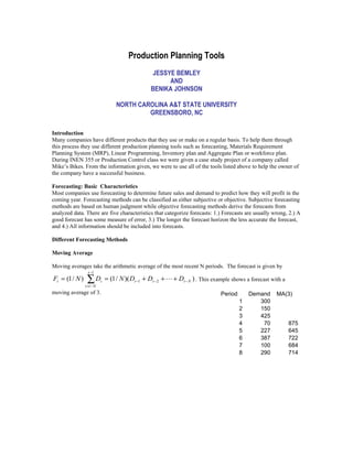
  • 1. Production Planning Tools JESSYE BEMLEY AND BENIKA JOHNSON NORTH CAROLINA A&T STATE UNIVERSITY GREENSBORO, NC Introduction Many companies have different products that they use or make on a regular basis. To help them through this process they use different production planning tools such as forecasting, Materials Requirement Planning System (MRP), Linear Programming, Inventory plan and Aggregate Plan or workforce plan. During INEN 355 or Production Control class we were given a case study project of a company called Mike’s Bikes. From the information given, we were to use all of the tools listed above to help the owner of the company have a successful business. Forecasting: Basic Characteristics Most companies use forecasting to determine future sales and demand to predict how they will profit in the coming year. Forecasting methods can be classified as either subjective or objective. Subjective forecasting methods are based on human judgment while objective forecasting methods derive the forecasts from analyzed data. There are five characteristics that categorize forecasts: 1.) Forecasts are usually wrong, 2.) A good forecast has some measure of error, 3.) The longer the forecast horizon the less accurate the forecast, and 4.) All information should be included into forecasts. Different Forecasting Methods Moving Average Moving averages take the arithmetic average of the most recent N periods. The forecast is given by t −1 Ft = (1 / N ) ∑D i =t − N i = (1 / N )( Dt −1 + Dt −2 +  + Dt − N ) . This example shows a forecast with a moving average of 3. Period Demand MA(3) 1 300 2 150 3 425 4 70 875 5 227 645 6 387 722 7 100 684 8 290 714
  • 2. Exponential Smoothing In exponential smoothing the current forecast is the weighted average of the last forecast and demand value. What is happening is NewForecast = α (Current observation of demand ) + (1 − α )( Last forecast ) . In symbols the equation would read Ft = αDt −1 + (1 − α ) Ft −1 . Period Demand ES(.1) 1 300 300 2 150 165 3 425 399 4 70 102.9 5 227 214.59 6 387 369.759 7 100 126.9759 8 290 273.6976 This table shows a forecast with an exponential smoothing constant of (.1). Regression Analysis Regression analysis fits a straight line over a set of data to show a trend. This straight line is computed by ˆ Y = a + bX . Next we have to determine the slope and intercept which can found by the next two S xy equations: b= ; a = D − b( n + 1) / 2 . To find our regression parameters we use: S xx n n( n + 1) n ∑ Di ; S xx = n (n + 16 2n + 1) − n (n4+ 1) . 2 2 2 )( S xy = n∑ iDi − i =1 2 i =1 Forecast for Mike’s Bikes For our project we used a subjective forecasting method called Winters’ Model. Winters’ Model is used for a seasonal series. Seasonal series have a pattern that repeats after some value of N periods. The Winters’ Model consists of three exponential smoothing equations that can be used as information is updated. The three equations represent the series, the trend and the seasonal factors. To begin the process we need initial estimates of at least two seasons. From this data we can calculate the sample means for both −N 0 1 1 sets of data. The calculations are as follows: V1 = N ∑ D j ; V2 = j = −2 N +1 N ∑D j = − N +1 j . Next, we define the initial slope that connects mean 1 to mean 2. This can be found by using this equation Go = (V2 − V1 ) / N . Then we find the estimated value of the series of time at time zero by the given equation S o = V2 + Go [( N − 10 / 2] . Last we determine the initial seasonal factors that can be computed for each period and then averaged to get the set seasonal factors. This equation calculates the seasonal factors Dt ct = . Vi − [( N + 1) / 2 − j ]Go
  • 3. Table 1. Below is an example of how we found each of these factors. 2005 Demand 110 117 V1= 122.5 127 113 133 2007 Demand 110 141 V2= 146 136 122 185 Go= 5.875 So= 154.8125 New C Norm. c-7 1.029137 c-3 1.028464 0.949089 c-6 1.117097 c-2 1.054221 0.972858 c-5 0.993953 c-1 0.992648 0.916038 c-4 1.169874 c-0 1.259196 1.162015 c-3 1.02779 Sum= 4.334529 4 c-2 0.991344 c-1 0.889294 c-0 1.348519 F 0,1 152.5068 F 0,2 162.0417 F 0,3 157.9593 F 0,4 207.2017 F 0,5 174.8104 F 0,6 184.9039 F 0,7 179.4862 F 0,8 234.5091 Aggregate Planning After being in business for a while companies need to take a look at their workforce and production line. Using an aggregate plan allows them to determine when to hire, fire workers and also determine the mix or quantity of products being manufactured. To begin making an aggregate plan we have to determine the aggregate unit. An aggregate unit is when items on a production line are similar. This can be calculated by Production rate/#of workers. There are two different plans you can use to calculate an aggregate plan zero inventory and constant workforce. A zero inventory plan changes the workforce each month in order to produce the amount of units that are close to demand pattern. A constant workforce plan tries to maintain a constant workforce to satisfy the net demand. For the purposes of our project we used the zero inventory plan. Under this plan we found the cumulative demand, number of aggregate units/ worker, minimum workers, workers hired, and workers fired. Once all these factors were calculated we can created a linear program to give us an optimal cost to see which model would be the best to use. There are many programs
  • 4. that can be used to create a linear program such as GAMS, LINGO, LINDO and Excel. Below is an example of the linear program we used to find the minimized cost using Microsoft Excel. MinC h ( H 1 + H 2 + H 3........) + C f ( F1 + F 2 + F 3 + .........) + C I ( I1 + I 2 + I 3 + ............) Subject to: I1= Inventory in stock + P1- Demand I2= I1 + P2 - Demand I3= I2 + P3 - Demand P1= W1*K*# of working days/month P2= W2*K*# of working days/month P3= W3*K*# of working days/month W1=beginning #of workers+ H1 - F1 W2= W1 + H2 - F2 W3=W2 + H3 - F3 I1>=buffer I2>=buffer I3>=buffer All variables>=0 Materials Requirements Planning System This systems allows personnel to plan when materials should arrive that are needed to make certain products. There are three phases to this system. The first phase is getting the information needed to make the Master Production Plan also known as a Bill of Materials. This shows the amounts and timing of production for each item. Figure 1. Shows an example of a Bill of Materials. 110 A(2) C(1) D(2) E(3) Lead Lot On Safety Item time Size Hand Allocation Stock 110 3 1 31 10 20 A 2 50 56 0 30
  • 5. C 1 50 23 0 10 D 2 150 118 0 100 E 1 250 160 0 150 Table 2. Shows the amount and timing of items produced. The next phase of the MRP is to determine the amount of planned ordered receipts. Phase 3 is the development of detailed shop floor schedules and resources requirements based on the planned order receipts. Below is an example of the MRP. Safety Stock Lead Time Low level Allocated On Hand Lot Size Item PD 1 2 3 4 5 6 7 8 Gross requirements 0 0 0 0 0 0 0 235 Scheduled receipts 0 0 0 0 0 0 0 0 Projected on hand 1 1 1 1 1 1 1 1 0 1 3 31 20 10 0 110 Net requirements 0 0 0 0 0 0 0 234 Planned order receipts 0 0 0 0 0 0 0 234 Planned order releases 0 0 0 0 234 0 0 0 PD 1 2 3 4 5 6 7 8 Gross requirements 0 0 0 0 0 0 0 431 Scheduled receipts 0 0 0 0 0 0 0 0 Projected on hand 2 2 2 2 2 2 2 2 0 1 4 22 20 0 0 210 Net requirements 0 0 0 0 0 0 0 429 Planned order receipts 0 0 0 0 0 0 0 429 Planned order releases 0 0 0 429 0 0 0 0 PD 1 2 3 4 5 6 7 8 Gross requirements 0 0 0 0 468 0 0 0 Scheduled receipts 0 0 0 0 0 0 0 0 Projected on hand 26 26 26 26 26 8 8 8 8 50 2 56 30 0 1 A Net requirements 0 0 0 0 442 0 0 0 Planned order receipts 0 0 0 0 450 0 0 0 Planned order releases 0 0 450 0 0 0 0 0 PD 1 2 3 4 5 6 7 8 Gross requirements 0 0 0 1716 0 0 0 0 Scheduled receipts 0 0 0 0 0 0 0 0 Projected on hand 28 28 28 28 28 28 28 28 28 100 2 78 50 0 1 B Net requirements 0 0 0 1688 0 0 0 0 Planned order receipts 0 0 0 1700 0 0 0 0 Planned order releases 1700 0 0 0 0 0 0 0 PD 1 2 3 4 5 6 7 8 Gross requirements 0 0 900 0 234 0 0 0 Scheduled receipts 0 0 0 0 0 0 0 0 Projected on hand 13 13 13 13 13 29 29 29 29 50 1 23 10 0 1 C Net requirements 0 0 887 0 221 0 0 0 Planned order receipts 0 0 900 0 250 0 0 0 Planned order releases 0 900 0 250 0 0 0 0 PD 1 2 3 4 5 6 7 8 Gross requirements 0 1800 0 500 0 0 0 50 Scheduled receipts 0 0 0 0 0 0 0 0 Projected on hand 18 18 18 18 118 118 118 118 68 150 2 118 100 0 2 D Net requirements 0 1782 0 482 0 0 0 0 Planned order receipts 0 1800 0 600 0 0 0 0 Planned order releases 0 0 0 0 0 0 0 0 PD 1 2 3 4 5 6 7 8 Gross requirements 0 1800 0 750 0 0 0 50 Scheduled receipts 0 0 0 0 0 0 0 0 Projected on hand 10 10 210 210 210 210 210 210 160 250 1 160 150 0 2 E Net requirements 0 1790 0 540 0 0 0 0 Planned order receipts 0 2000 0 750 0 0 0 0 Planned order releases 0 0 0 0 0 0 0 0 PD 1 2 3 4 5 6 7 8 Inventory Control Basics of Inventory It is important for businesses or companies to keep a record of what items or products they have in inventory. Inventory can be classified into four different types raw materials, components, Work-in- process, and finished goods. Raw materials are the resources needed to produce a product. Components are either raw materials or subassemblies that will be included in the final product. Work-in-process is inventory in the plant waiting to be processed. Finished goods are completed and waiting to be shipped out to distributors. There are different characteristics that describe inventory systems such as pattern of
  • 6. demand, replenishment lead times, review times, and treatment of excess demand. The pattern of demand can either be a constant versus variable which assumes that the demand is constant and the known versus random assumes the demand is constant but still random which means it still has some uncertainty. The lead time tells us the exact amount of time it takes to receive an item from when its order was placed. Review time allows time to accurately record inventory levels at all times. Excess demand is how the system reacts to having more inventory than the systems can handle. Three different costs are associated with inventory holding, order, and penalty costs. These costs are used to help with different inventory models to minimize costs. Different Inventory Models Economic Order Quantity One model that is used for known demand is the Economic Order Quantity Model or (EOQ). This system deals with products that are already made to buy. This model assumes that the demand is known and constant. Shortages are not permitted. There is no order lead time. It has setup, order and holding costs. The basic job for this model is to determine the optimal quantity order or Q*. First, the total annual cost is Kλ hQ calculated G (Q ) = + λc + . From this we can find the optimal Q* by using this equation Q 2 2 Kλ Q* = . h Quantity Discount Model In the EOQ model cost is independent of the size of the order. But, using the quantity discount model the supplier will charge less based on the retailer or customer buying a higher batch of products. There are two types of discounts that can be applied to all units, fixed and incremental which applies the discount to anything addition or beyond the breakpoint. All units use a similar equation like the EOQ but has, a fixed order cost and interest rate defined as: G j (Q) = λc j + λK / Q + Ic j Q / 2 . The incremental discount uses a piece wise type of function and the Go (Q) for 0 ≤ Q < t  G (Q) = G1 (Q) for t ≤ Q < u same order quantity function: G (Q) .  2 for u ≤ Q
  • 7. Inventory Plan To keep an accurate record you need to know the demand, certain costs, the mean demand during lead time and standard deviation. These factors are key to helping us determine the order quantity of items, the reorder point, safety stock and the value of asset pooling. Given the data below for six distributors we created an accurate Inventory plan for Mike’s Bikes. East Seast Midwest West Mtn Nwest Model 110 Annual Demand 58 117 88 105 123 94 Model 210 Annual Demand 90 180 135 162 189 144 Order cost( both bikes ordered together) $1,000 $800 $800 $1,400 $1,000 $1,500 Annual Holding Cost (same for both models) $326 $403 $387 $391 $249 $390 Total Model 110 Mean Demand During Leadtime 19.3 39 29.3 35 41 31.3 194.9 Model 110 Demand Std. Dev. During Leadtime 0.49 14.12 14.21 9.59 6.15 3.02 47.58 Model 210 Mean Demand During Leadtime 30 60 45 54 63 48 300 Model 210 Demand Std. Dev. During Leadtime 8.65 4.9 19.47 0.94 27.76 0.49 62.21 As discussed earlier in different inventory plans was the order quantity which can be found using the optimal Q* equation. Then we determine the reorder point which is the point where the inventory on hand is getting low and an order should be placed. We determine the reorder point by using this equation: R = λ + Z α σ . We chose to use a 95% confidence interval because we wanted to consider only 5% of error in the bikes made. The safety stock is the extra products that are left in stock this can be defined as: SS = Z α σ .The value of asset pooling allows different companies to pull from each others inventory if they do not have a particular product. We determine this amount by using the same data as the safety stock. All of our results were found using Microsoft Excel and are shown below. 19.0741 Order Quanity Model 110 18.86341 21.55264 8 27.42113 31.4317 26.89009 23.6249 38.9624 Order Quanity Model 210 23.49781 26.73276 8 34.06027 5 33.28201 Reorder point Model 110 20.1036 62.1568 52.6044 50.7276 51.086 36.2528 108.526 Reorder point Model 210 44.186 68.036 76.9308 55.5416 4 48.8036 Total Safety Stock for Model 110 0.8036 23.1568 23.3044 15.7276 10.086 4.9528 78.0312 102.024 Safety Stock for Model 210 14.186 8.036 31.9308 1.5416 45.5264 0.8036 4 ALL Ware. 468.1872 612.1464 Value of Asset Poolin for Model 110 78.0312 Value of Asset Poolin for Model 210 102.0244
  • 8. Results Table 3 shows the original data provided for the case study. Based on the data given for Mike’s Bike Shop, our process consisted of generating a forecast, workforce plan and MRP for the next two years. Our method selection for forecasting was Winters Model because of the seasonal trend in the initial demand from the previous years. We chose to forecast the future based on the first year and the final year of demand. The workforce plan was generated using a zero inventory plan and compared with a linear program that solved the workforce plan optimally. In the provided workbook set, the aggregate unit for each model was determined by solving for the average production rate and the number of workers. Based on the defined aggregate units for both models, Mike can determine his quarterly workforce needed. The linear program consisted of four major constraints and five variable components. This allowed us to minimize the cost to hold inventory, hire workers, and fire workers for each model. The MRP was concluded by combining both Bills of Materials needed to produce both models. We used both models because both models had similar products in order to be considered a finished good. The initial gross requirements were also the final forecasted demand for the last year. From there, we were able to find the actual amount of materials required in order to meet the scheduled plan. Finally, the inventory plan consisted of six distributors defined by regions. From the data given, we were able to determine the reorder point, order quantity, safety stock, and the value of asset pooling. Using EOQ, the order quantity was able to be computed. EOQ was the selection of choice because the parts were being bought instead of being made which is used in EPQ. Using a confidence interval of 95%, the reorder point for both models this would assist Mike with his inventory plan.
  • 9. Conclusion Production Planning Tools can be used in everyday companies to help provide better efficient services. Each of these techniques are easy to use and can be done with different software programs such as Excel, GAMS, LINDO and LINGO. These tools help companies to look at their overall business and make changes that will save them money, create safer environments, create a better production line, plan efficient scheduling and be aware of inventory coming and going out. As shown through the Case Study on Mike’s Bikes the techniques work and show that any company can be successful but save money. Reference Nahmias, Steven. Production and Operations Anaylsis. New York, McGraw Hill. 2005