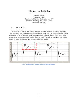
1. 1
EE 481 – Lab #6
Mireille Mballa
Chad Ryan Weiss
Department of Electrical Engineering and EET
Penn State Harrisburg, The Capitol College
Middletown, PA 17057
I. OBJECTIVES
The objective of this lab is to examine different methods to control the robotic arm called
“pick and place”. Fig. 1 shows the open loop response of the arm. The move in this case is along
an arc from 30° to 60° compare to the robot manipulator reference frame. Fig. 2 shows more
details on the open loop response moving from 30° to 60°. We will use our closed loop control
system to “filter” the step function to obtain satisfactory results.
Fig. 1: Uncontrolled pick and place robotic arm open loop response

2. 2
II. METHODS
We used the step response in Fig. 2 to find the open loop plant transfer function, G(s). Equation (1) is
the format of the transfer function that we need to find.
𝐺( 𝑠) =
ω 𝑛
2
𝑆2 + 2ζ ω 𝑛 𝑠 +ω 𝑛
2
In order to find different coefficient of the equation, we did some alternate calculations using Fig. 2,
we were able to assume that the peak time Tp=1.162s with the value of the peak time, we found ωd using
equation (2). We also needed to find ζ we used equation (3) to find that value and with the values
of ωd and ζ, equation (4) were used to find ωn.
T𝑝 =
𝜋
ω 𝑑
ω 𝑑 = 19.4
%𝑂𝑆 = 100 ∗ 𝑒
−𝜋(
𝜁
√1−𝜁2
)
With %𝑂𝑆 =
73.3−60
30
∗ 100 = 44.3 we have 𝝵=.25
𝜔 𝑛 =
ω 𝑑
√1 − 𝜁2
𝜔 𝑛 = 20
Fig. 2 Detail of open loop response of arm moving from 30° to 60°
(1)
(2)
(3)
(4)

3. 3
The transfer function of the plant is G(s) =
400
𝑠2+10𝑠+400
Now to make sure we found the right transfer function of the plant, we simulated our
function in Simulink using Fig. 3 below. We made sure that one of the pulse generator is set for
an amplitude of 30, period of 2 seconds, duty cycle of 50%, and no phase delay. The second
pulse generator is set to an amplitude of 60, period of 2, duty cycle of 50%, and phase delay of 1
second.
Fig.3. Input scheme for plant testing
The result of the simulation is shown in Fig. 4 and Fig. 5 show a closed up of the open loop
response using the transfer function found.
Fig. 4: Open loop response using the transfer function found while doing calculations
Fig. 5: Close up of the open loop response using the transfer function found while doing calculations

4. 4
After evaluating both Fig. 4 and Fig. 5, we can proceed with confidence through the lab as
our transfer function is correct. We obtained the same graphs as the ones given during the lab
and we calculated and compared our values found for the rise time, peak time, settling time, and
steady state error. Equations (5) and (6), (7) were used to find those values.
T𝑝 =
𝜋
ω 𝑑
T𝑝 = 1 + 0.162
We added due to the offset since the first second is the initial pulse.
T𝑝 = 1.162𝑠
𝑇𝑠 = 60𝑠
The settling time was based on the graph shown in Fig. 5.
𝑇𝑟 = 1.23𝑠
𝑒𝑠𝑡𝑎𝑡𝑒 =
1
1 + 𝑘 𝑝
𝑒𝑠𝑡𝑎𝑡𝑒 = 0.5
We looked at the difference between the final value when the amplitude of 30 and the amplitude
of 60 and we obtain a difference of .5.
We closed the loop on the system and found the transfer function T(s). We used the equation (7)
𝑇( 𝑠) =
𝐾𝐺(𝑠)
1 + 𝐺(𝑠)
Which lead to the final answer of: 𝑇( 𝑠) =
𝐾∗400
𝑠2+10𝑠+400(𝑘+1)
We also found the root locus using the Matlab script in Fig. 6. The graph obtain is shown in Fig.
7.
Fig.6: Matlab script of the root locus
(5)
(7)
(7)
(6)

5. 5
Fig. 7: Root locus of the transfer function T(s)
To determine whether or not it is possible for the proportional control in Fig. 8 to be
improved to the overshoot of 5%, we used equations (8) and (9) to find Kp and steady state error,
when we simulated our values on Matlab, we realized that its was not possible to improve to 5%
because as the value of the gain increased, the steady state error was increased instead of
decreasing.
𝐾𝑝 =
400𝐾
400(𝐾+1)
and 𝑒𝑠𝑡𝑎𝑡𝑖𝑐 =
1
1+𝐾 𝑝
𝑒 𝑠𝑡𝑎𝑡𝑖𝑐 =
400𝐾 + 400
800𝐾 + 400
Fig. 8: Proportional control scheme
In order for the pick and place end to work properly, the settling time for the response
was modified to 5%. Using the equations (3),(10), and (11), we were able to find a set of
dominant target poles positions that will make the pick and place work properly at a settling time
of .4s.
(9)
(8)

6. 6
𝑇𝑠 = .4𝑠
𝑇𝑠 =
4
𝑥
𝑥 = 10
𝜔 𝑛 =
𝑥
𝜁
With %𝑂𝑆 = 5%
𝜁 = .69
𝜔 𝑛 = 14.5
Knowing that the format of the poles is: -𝝵𝞈n ±j𝞈n√1 − 𝜁2 we conclude that the new
dominant target pole is: -10±j10.5.
We then designed a Proportional Controller, PD controller, PID controller, and a hybrid
controller to determine whether the desired pole could be achieved by the system without
compromising stability.
III. Results
The first system that was created was a proportional control system. Looking at the figure
below we see that the result of our system was stable but did not have the desired system
characteristics that we were looking for.
Figure 9: Proportional Control Waveform
(11)
(10)

7. 7
The desired system parameters include a 5% overshoot and a settling time of 0.4 seconds.
Using the root locus command in Matlab allows us to see the exact trajectory of our system and
from that trajectory we can determine if our controller will give us the desired parameters. See
Fig. 10.
Figure 10: Proportional Control Root Locus
As noticed in Fig. 10, the root locus clearly shows that the proportional controller cannot,
under any circumstances, yield a 5% overshoot and hence, this type of control scheme will not
work for our system.
The next control scheme to be implemented was a PD controller. The figure below shows
a condensed version of the block diagram of the system.
Figure 11: Condensed PD Control System
The resulting waveform of this system shows that the PD controller did not help the
cause at all and in fact made it worse, see Fig. 12. and Fig. 13.

8. 8
Figure 12: PD Controller Waveform
Figure 13: PD Controller Root Locus
Fig. 12 and Fig. 13 clearly show that the PD control scheme will not give us the desired
system parameters. The PID controller, shown in Fig. 14 will also make no real difference as far
as the system parameters go.
Figure 14: Condensed PID Control System

9. 9
Fig. 14 shows a condensed version of the PID control system. The only difference is that
a zero was added at -0.1 and a pole at zero. See Fig. 15 for the resulting waveform.
Figure 15: PID Controller Waveform
As seen in Fig. 15 the added zero and pole did not help the system in any way
whatsoever; however, it is important to notice that the system has now gone from stable to
unstable as it continues to grow in the negative direction without bound.
Figure 16: PID Control Root Locus
As seen in Fig. 16, the newly added pole and zero to the system did not help our case
when it comes to achieving the desired system parameters. Hence, our next control mechanism
will be a completely new approach altogether. We will call this scheme the hybrid control
mechanism. See Fig. 17.

10. 10
Figure 17: Hybrid Control Mechanism
Fig. 17 shows the controller that will ultimately give us the desired system parameters
without compromising stability. The control signal block shown as Transfer Fcn1 will act as the
system controller and the other block labeled, Transfer Fcn represents the original system plant.
Our control signal consists of two poles and two zeros. One of the poles happens to be located at
the origin and another at a location that was obtained through trigonometry, i.e. lead
compensation. The two zeros that were implemented in our control system were placed at the
location of the original poles to make the calculations simpler. Therefore, after tedious
calculation, we came up with the following result.
Figure 18: Hybrid Controller Waveform
As seen in Fig. 18, the hybrid controller waveform has the qualities and characteristics
that consummate the objective of this lab. The percent overshoot was reduced to 5% and the
settling time was reduced to 0.4 seconds due to the new target poles.

11. 11
Figure 19: Hybrid ControllerRoot Locus
Furthermore, the root locus diagram shown in Fig. 19 shows us that the percent overshoot
is in fact 5% at the desired target pole location. Hence, it is safe to say that this control
mechanism was the one that proved effective for the purposes of our experiment.
Summary:
Based on the root locus for proportional control, it is not possible to reduce percent
overshoot through proportion control only because it will be difficult to obtain simple gain with a
plant with no zeros.
The PD controller did not deliver the results we expected because our dominant real part
would have been -1.25 which when we look at the root locus in Fig.13, it would have been
impossible. Also, the predicted steady state is 0.75, but with this controller it is 1. There were no
improvements with the PID controller because the stability of the system is affected. The system
went from a stable system to an unstable system.
The hybrid controller worked well because it used the lead compensation to cancel an
undesirable pole and at the same time kept the order of the denominator the same which did not
compromise the stability of the system.
Based on our observations, we realized that the best situation for using the proportional
control is on active circuits when we want to improve the steady state error only. The best
situations to use the PD control is on active circuits when we want to improve the transient
response only. The best situation to use the PID controller is on active circuits when we want to
improve both the transient response and the steady state error and implement an additional pole
to cancel the noise and saturation.
The hybrid controller is better when we want to use the lead compensation technique in
order to meet the system requirements. The disadvantage of the hybrid controller is that it
requires the use of two poles and two zeros that changes the system type.
If we are in the situation where we could not use an active circuit to produce a pure pole
at zero, we can use the lead-lag compensation controller. This controller does not require active
circuits. It is also implemented in passive circuit and it also improves the steady state error and
the transient response.
IV. Conclusions

12. 12
In conclusion, we used different methods to control a robotic arm called “pick and place”
which is a simple move use by industrial robots to pick up an object and place it in another
location. The move long the arc in his case is from 30° to 60° compare to the robot manipulator.
Since the first move is done from 0° to 30°, we tried different controllers during the lab to
determine which controller will allow the arm robot to do the movement with a 5% overshoot
and a settling time of 0.4s. After trying the proportional control, the PD, the PID, and the hybrid
controllers, the only controller that meets the requirements is the hybrid controller as the other
controllers either affect only the steady state error or just the transient response.
V. References
[1] N. Nise, Control Systems Engineering, 6th edition. New Jersey, Wiley, 2011, pp. 456-494.
[2] S. van Tonningen, “EE 481- Lecture note week 9: Static Error Constants” Course handout,
2015.
[3] S. van Tonningen, “EE 481- Lecture note week 10: Root Locus” Course handout, 2015.
[4] S. van Tonningen, “EE 481- Lecture note week 11: PI Control” Course handout, 2015.
[5] S. van Tonningen, “EE 481 – Laboratory 7: Practicing Varioius Control Techniques” Course
Handout, 2015.