This is supporting material for the presentation https://www.slideshare.net/CodeOps/big-data-analytics-with-matlab.

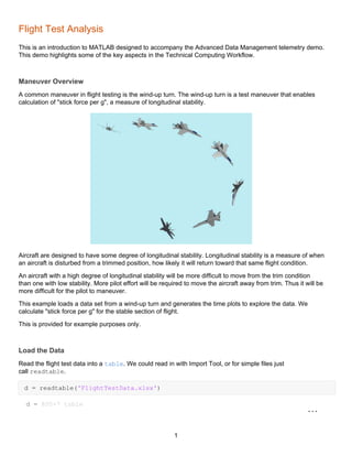
1. Flight Test Analysis
This is an introduction to MATLAB designed to accompany the Advanced Data Management telemetry demo.
This demo highlights some of the key aspects in the Technical Computing Workflow.
Maneuver Overview
A common maneuver in flight testing is the wind-up turn. The wind-up turn is a test maneuver that enables
calculation of "stick force per g", a measure of longitudinal stability.
Aircraft are designed to have some degree of longitudinal stability. Longitudinal stability is a measure of when
an aircraft is disturbed from a trimmed position, how likely it will return toward that same flight condition.
An aircraft with a high degree of longitudinal stability will be more difficult to move from the trim condition
than one with low stability. More pilot effort will be required to move the aircraft away from trim. Thus it will be
more difficult for the pilot to maneuver.
This example loads a data set from a wind-up turn and generates the time plots to explore the data. We
calculate "stick force per g" for the stable section of flight.
This is provided for example purposes only.
Load the Data
Read the flight test data into a table. We could read in with Import Tool, or for simple files just
call readtable.
d = readtable('FlightTestData.xlsx')
d = 800×7 table
1

2. Time AirSpeed AoA BankAngle Elevator LoadFactor
1 0.5312 249.4890 2.2690 33.3510 -1.9550 1.1679
2 0.5313 249.4890 2.2690 33.3510 -1.9550 1.1704
3 0.5313 249.4890 2.2690 33.3510 -1.9550 1.1660
4 0.5313 249.4890 2.2690 33.3510 -1.9550 1.1837
5 0.5313 249.4889 2.2690 33.3510 -1.9550 1.2234
6 0.5313 249.4889 2.2690 33.3510 -1.9550 1.2318
7 0.5313 249.4889 2.2690 33.3510 -1.9550 1.2306
8 0.5313 249.4889 2.2690 33.3510 -1.9550 1.2312
9 0.5313 249.4889 2.2690 33.3510 -1.9550 1.2297
10 0.5313 249.4889 2.2690 33.3509 -1.9550 1.2230
11 0.5313 249.4889 2.2690 33.3509 -1.9550 1.2113
12 0.5313 249.4888 2.2690 33.3509 -1.9551 1.1942
13 0.5313 249.4888 2.2690 33.3509 -1.9551 1.1736
14 0.5313 249.4888 2.2690 33.3509 -1.9551 1.1533
15 0.5313 249.4888 2.2690 33.3509 -1.9551 1.1330
16 0.5313 249.4888 2.2690 33.3509 -1.9551 1.1125
17 0.5313 249.4888 2.2690 33.3509 -1.9551 1.0929
18 0.5313 249.4888 2.2690 33.3509 -1.9551 1.0775
19 0.5313 249.4887 2.2690 33.3509 -1.9551 1.0673
20 0.5313 249.4887 2.2690 33.3509 -1.9551 1.0623
21 0.5313 249.4887 2.2690 33.3509 -1.9551 1.0614
22 0.5313 249.4887 2.2690 33.3509 -1.9551 1.0615
23 0.5313 249.4887 2.2690 33.3509 -1.9551 1.0615
24 0.5313 249.5262 2.2691 33.3509 -1.9551 1.0615
25 0.5313 249.6059 2.2691 33.3509 -1.9551 1.0615
26 0.5313 249.6857 2.2691 33.3508 -1.9551 1.0615
27 0.5313 249.7654 2.2696 33.3508 -1.9551 1.0615
28 0.5313 249.8452 2.2717 33.3508 -1.9551 1.0615
29 0.5313 249.9249 2.2739 33.3508 -1.9551 1.0615
30 0.5313 249.9269 2.2761 33.3508 -1.9551 1.0615
31 0.5313 249.9269 2.2783 33.3508 -1.9551 1.0615
32 0.5313 249.9269 2.2805 33.3508 -1.9551 1.0615
2

3. Time AirSpeed AoA BankAngle Elevator LoadFactor
33 0.5313 249.9269 2.2827 33.3508 -1.9552 1.0615
34 0.5313 249.9269 2.2848 33.3508 -1.9552 1.0615
35 0.5313 249.9269 2.2870 33.3508 -1.9552 1.0615
36 0.5313 249.9192 2.2892 33.3508 -1.9552 1.0615
37 0.5313 249.8483 2.2942 33.3508 -1.9552 1.0615
38 0.5313 249.7774 2.2995 33.3508 -1.9552 1.0615
39 0.5313 249.7066 2.3049 33.3508 -1.9552 1.0615
40 0.5313 249.6357 2.3102 33.3508 -1.9552 1.0615
41 0.5313 249.6138 2.3156 33.3508 -1.9552 1.0615
42 0.5313 249.5925 2.3209 33.3507 -1.9552 1.0615
43 0.5313 249.5712 2.3263 33.3507 -1.9552 1.0615
44 0.5313 249.5500 2.3317 33.3507 -1.9552 1.0615
45 0.5313 249.5287 2.3370 33.3507 -1.9552 1.0615
46 0.5313 249.5074 2.3424 33.3507 -1.9551 1.0615
47 0.5313 249.4824 2.3477 33.3507 -1.9554 1.0615
48 0.5313 249.4292 2.3516 33.3507 -1.9569 1.0615
49 0.5313 249.3760 2.3536 33.3507 -1.9593 1.0615
50 0.5313 249.3229 2.3555 33.3507 -1.9614 1.0615
51 0.5313 249.2697 2.3575 33.3507 -1.9637 1.0615
52 0.5313 249.2165 2.3594 33.3507 -1.9659 1.0615
53 0.5313 249.1634 2.3614 33.3507 -1.9681 1.0615
54 0.5313 249.1102 2.3634 33.4925 -1.9703 1.0615
55 0.5313 249.0570 2.3653 33.6849 -1.9725 1.0615
56 0.5313 249.0319 2.3673 33.8774 -1.9746 1.0615
57 0.5313 249.0106 2.3693 34.0699 -1.9773 1.0615
58 0.5313 248.9893 2.3711 34.2624 -1.9765 1.0615
59 0.5313 248.9681 2.3711 34.4549 -1.9706 1.0615
60 0.5313 248.9468 2.3711 34.6474 -1.9657 1.0615
61 0.5313 248.9255 2.3711 34.8399 -1.9606 1.0615
62 0.5313 248.9045 2.3711 35.0324 -1.9555 1.0615
63 0.5313 248.9045 2.3711 35.2249 -1.9504 1.0615
64 0.5313 248.9045 2.3711 35.4174 -1.9453 1.0615
3

4. Time AirSpeed AoA BankAngle Elevator LoadFactor
65 0.5313 248.9045 2.3711 35.6045 -1.9402 1.0615
66 0.5313 248.9045 2.3711 35.7906 -1.9351 1.0615
67 0.5313 248.9045 2.3711 35.9767 -1.9300 1.0615
68 0.5313 248.9045 2.3711 36.1629 -1.9249 1.0615
69 0.5313 248.9026 2.3711 36.3490 -1.9198 1.0615
70 0.5313 248.8893 2.3711 36.5352 -1.9146 1.0615
71 0.5313 248.8760 2.3711 36.7213 -1.9100 1.0615
72 0.5313 248.8627 2.3711 36.9075 -1.9076 1.0615
73 0.5313 248.8494 2.3711 37.0936 -1.9062 1.0615
74 0.5313 248.8361 2.3711 37.3533 -1.9046 1.0615
75 0.5313 248.8314 2.3711 37.7679 -1.9030 1.0615
76 0.5313 248.8314 2.3711 38.1825 -1.9014 1.0615
77 0.5313 248.8314 2.3711 38.5971 -1.8998 1.0615
78 0.5313 248.8314 2.3711 38.9692 -1.8983 1.0615
79 0.5313 248.8314 2.3711 39.2061 -1.8967 1.0615
80 0.5313 248.8314 2.3711 39.4430 -1.8951 1.0615
81 0.5313 248.8314 2.3708 39.6799 -1.8935 1.0615
82 0.5313 248.8314 2.3686 39.9168 -1.8919 1.0615
83 0.5313 248.8314 2.3664 40.1538 -1.8904 1.0615
84 0.5313 248.8311 2.3642 40.3279 -1.8887 1.0615
85 0.5313 248.8205 2.3621 40.4858 -1.8873 1.0615
86 0.5313 248.8098 2.3599 40.6437 -1.8850 1.0615
87 0.5313 248.7992 2.3577 40.8017 -1.8811 1.0615
88 0.5313 248.7886 2.3555 40.9596 -1.8775 1.0615
89 0.5313 248.7779 2.3533 41.1176 -1.8738 1.0615
90 0.5313 248.7673 2.3511 41.2755 -1.8702 1.0615
91 0.5313 248.7584 2.3547 41.4334 -1.8661 1.0615
92 0.5313 248.7584 2.3596 41.5665 -1.8645 1.0615
93 0.5313 248.7584 2.3645 41.6850 -1.8682 1.0615
94 0.5313 248.7584 2.3694 41.8034 -1.8727 1.0615
95 0.5313 248.7584 2.3690 41.9219 -1.8771 1.0616
96 0.5313 248.7584 2.3657 42.0403 -1.8815 1.0612
4

5. Time AirSpeed AoA BankAngle Elevator LoadFactor
97 0.5313 248.7584 2.3625 42.1588 -1.8859 1.0631
98 0.5313 248.7584 2.3592 42.2772 -1.8903 1.0754
99 0.5313 248.7584 2.3559 42.3957 -1.8947 1.1016
100 0.5313 248.7584 2.3526 42.5142 -1.8992 1.1417
Visualize Airspeed
Plots appear directly in the Live Editor. You can interactively pan, zoom, and rotate plots and generate
MATLAB code to capture the final view.
plot(d.AirSpeed)
xlim([138 276])
ylim([246.45 251.70])
Convert Times to datetime
5

6. Our dates are stored as an offset from a particular point in time in Excel. MATLAB can use this method or
store dates in a container called a datetime which provides a number of useful features for working with
time data such as easy ways to handle time zone changes, leap years, and calculating durations.
d.Time = datetime(d.Time, 'ConvertFrom', 'Excel','Format','hh:mm:ss.SSS a')
d = 800×7 table
Time AirSpeed AoA BankAngle Elevator LoadFactor
1 12:45:00.00... 249.4890 2.2690 33.3510 -1.9550 1.1679
2 12:45:00.05... 249.4890 2.2690 33.3510 -1.9550 1.1704
3 12:45:00.10... 249.4890 2.2690 33.3510 -1.9550 1.1660
4 12:45:00.15... 249.4890 2.2690 33.3510 -1.9550 1.1837
5 12:45:00.20... 249.4889 2.2690 33.3510 -1.9550 1.2234
6 12:45:00.25... 249.4889 2.2690 33.3510 -1.9550 1.2318
7 12:45:00.30... 249.4889 2.2690 33.3510 -1.9550 1.2306
8 12:45:00.35... 249.4889 2.2690 33.3510 -1.9550 1.2312
9 12:45:00.40... 249.4889 2.2690 33.3510 -1.9550 1.2297
10 12:45:00.45... 249.4889 2.2690 33.3509 -1.9550 1.2230
11 12:45:00.50... 249.4889 2.2690 33.3509 -1.9550 1.2113
12 12:45:00.55... 249.4888 2.2690 33.3509 -1.9551 1.1942
13 12:45:00.60... 249.4888 2.2690 33.3509 -1.9551 1.1736
14 12:45:00.65... 249.4888 2.2690 33.3509 -1.9551 1.1533
15 12:45:00.70... 249.4888 2.2690 33.3509 -1.9551 1.1330
16 12:45:00.75... 249.4888 2.2690 33.3509 -1.9551 1.1125
17 12:45:00.80... 249.4888 2.2690 33.3509 -1.9551 1.0929
18 12:45:00.85... 249.4888 2.2690 33.3509 -1.9551 1.0775
19 12:45:00.90... 249.4887 2.2690 33.3509 -1.9551 1.0673
20 12:45:00.95... 249.4887 2.2690 33.3509 -1.9551 1.0623
21 12:45:01.00... 249.4887 2.2690 33.3509 -1.9551 1.0614
22 12:45:01.05... 249.4887 2.2690 33.3509 -1.9551 1.0615
23 12:45:01.10... 249.4887 2.2690 33.3509 -1.9551 1.0615
24 12:45:01.15... 249.5262 2.2691 33.3509 -1.9551 1.0615
25 12:45:01.20... 249.6059 2.2691 33.3509 -1.9551 1.0615
26 12:45:01.25... 249.6857 2.2691 33.3508 -1.9551 1.0615
27 12:45:01.30... 249.7654 2.2696 33.3508 -1.9551 1.0615
6

7. Time AirSpeed AoA BankAngle Elevator LoadFactor
28 12:45:01.35... 249.8452 2.2717 33.3508 -1.9551 1.0615
29 12:45:01.40... 249.9249 2.2739 33.3508 -1.9551 1.0615
30 12:45:01.45... 249.9269 2.2761 33.3508 -1.9551 1.0615
31 12:45:01.50... 249.9269 2.2783 33.3508 -1.9551 1.0615
32 12:45:01.55... 249.9269 2.2805 33.3508 -1.9551 1.0615
33 12:45:01.60... 249.9269 2.2827 33.3508 -1.9552 1.0615
34 12:45:01.65... 249.9269 2.2848 33.3508 -1.9552 1.0615
35 12:45:01.70... 249.9269 2.2870 33.3508 -1.9552 1.0615
36 12:45:01.75... 249.9192 2.2892 33.3508 -1.9552 1.0615
37 12:45:01.80... 249.8483 2.2942 33.3508 -1.9552 1.0615
38 12:45:01.85... 249.7774 2.2995 33.3508 -1.9552 1.0615
39 12:45:01.90... 249.7066 2.3049 33.3508 -1.9552 1.0615
40 12:45:01.95... 249.6357 2.3102 33.3508 -1.9552 1.0615
41 12:45:02.00... 249.6138 2.3156 33.3508 -1.9552 1.0615
42 12:45:02.05... 249.5925 2.3209 33.3507 -1.9552 1.0615
43 12:45:02.10... 249.5712 2.3263 33.3507 -1.9552 1.0615
44 12:45:02.15... 249.5500 2.3317 33.3507 -1.9552 1.0615
45 12:45:02.20... 249.5287 2.3370 33.3507 -1.9552 1.0615
46 12:45:02.25... 249.5074 2.3424 33.3507 -1.9551 1.0615
47 12:45:02.30... 249.4824 2.3477 33.3507 -1.9554 1.0615
48 12:45:02.35... 249.4292 2.3516 33.3507 -1.9569 1.0615
49 12:45:02.40... 249.3760 2.3536 33.3507 -1.9593 1.0615
50 12:45:02.45... 249.3229 2.3555 33.3507 -1.9614 1.0615
51 12:45:02.50... 249.2697 2.3575 33.3507 -1.9637 1.0615
52 12:45:02.55... 249.2165 2.3594 33.3507 -1.9659 1.0615
53 12:45:02.60... 249.1634 2.3614 33.3507 -1.9681 1.0615
54 12:45:02.65... 249.1102 2.3634 33.4925 -1.9703 1.0615
55 12:45:02.70... 249.0570 2.3653 33.6849 -1.9725 1.0615
56 12:45:02.75... 249.0319 2.3673 33.8774 -1.9746 1.0615
57 12:45:02.80... 249.0106 2.3693 34.0699 -1.9773 1.0615
58 12:45:02.85... 248.9893 2.3711 34.2624 -1.9765 1.0615
59 12:45:02.90... 248.9681 2.3711 34.4549 -1.9706 1.0615
7

8. Time AirSpeed AoA BankAngle Elevator LoadFactor
60 12:45:02.95... 248.9468 2.3711 34.6474 -1.9657 1.0615
61 12:45:03.00... 248.9255 2.3711 34.8399 -1.9606 1.0615
62 12:45:03.05... 248.9045 2.3711 35.0324 -1.9555 1.0615
63 12:45:03.10... 248.9045 2.3711 35.2249 -1.9504 1.0615
64 12:45:03.15... 248.9045 2.3711 35.4174 -1.9453 1.0615
65 12:45:03.20... 248.9045 2.3711 35.6045 -1.9402 1.0615
66 12:45:03.25... 248.9045 2.3711 35.7906 -1.9351 1.0615
67 12:45:03.30... 248.9045 2.3711 35.9767 -1.9300 1.0615
68 12:45:03.35... 248.9045 2.3711 36.1629 -1.9249 1.0615
69 12:45:03.40... 248.9026 2.3711 36.3490 -1.9198 1.0615
70 12:45:03.45... 248.8893 2.3711 36.5352 -1.9146 1.0615
71 12:45:03.50... 248.8760 2.3711 36.7213 -1.9100 1.0615
72 12:45:03.55... 248.8627 2.3711 36.9075 -1.9076 1.0615
73 12:45:03.60... 248.8494 2.3711 37.0936 -1.9062 1.0615
74 12:45:03.65... 248.8361 2.3711 37.3533 -1.9046 1.0615
75 12:45:03.70... 248.8314 2.3711 37.7679 -1.9030 1.0615
76 12:45:03.75... 248.8314 2.3711 38.1825 -1.9014 1.0615
77 12:45:03.80... 248.8314 2.3711 38.5971 -1.8998 1.0615
78 12:45:03.85... 248.8314 2.3711 38.9692 -1.8983 1.0615
79 12:45:03.90... 248.8314 2.3711 39.2061 -1.8967 1.0615
80 12:45:03.95... 248.8314 2.3711 39.4430 -1.8951 1.0615
81 12:45:04.00... 248.8314 2.3708 39.6799 -1.8935 1.0615
82 12:45:04.05... 248.8314 2.3686 39.9168 -1.8919 1.0615
83 12:45:04.10... 248.8314 2.3664 40.1538 -1.8904 1.0615
84 12:45:04.15... 248.8311 2.3642 40.3279 -1.8887 1.0615
85 12:45:04.20... 248.8205 2.3621 40.4858 -1.8873 1.0615
86 12:45:04.25... 248.8098 2.3599 40.6437 -1.8850 1.0615
87 12:45:04.30... 248.7992 2.3577 40.8017 -1.8811 1.0615
88 12:45:04.35... 248.7886 2.3555 40.9596 -1.8775 1.0615
89 12:45:04.40... 248.7779 2.3533 41.1176 -1.8738 1.0615
90 12:45:04.45... 248.7673 2.3511 41.2755 -1.8702 1.0615
91 12:45:04.50... 248.7584 2.3547 41.4334 -1.8661 1.0615
8

9. Time AirSpeed AoA BankAngle Elevator LoadFactor
92 12:45:04.55... 248.7584 2.3596 41.5665 -1.8645 1.0615
93 12:45:04.60... 248.7584 2.3645 41.6850 -1.8682 1.0615
94 12:45:04.65... 248.7584 2.3694 41.8034 -1.8727 1.0615
95 12:45:04.70... 248.7584 2.3690 41.9219 -1.8771 1.0616
96 12:45:04.75... 248.7584 2.3657 42.0403 -1.8815 1.0612
97 12:45:04.80... 248.7584 2.3625 42.1588 -1.8859 1.0631
98 12:45:04.85... 248.7584 2.3592 42.2772 -1.8903 1.0754
99 12:45:04.90... 248.7584 2.3559 42.3957 -1.8947 1.1016
100 12:45:04.95... 248.7584 2.3526 42.5142 -1.8992 1.1417
Verify Airspeed Stability
For this data to be useful, the airspeed must remain relatively constant throughout the maneuver. Visually
inspect the data to ensure we are within 5 knots during the smooth section, or within 10 knots during the stall
buffet.
Compare airspeed with load factor over the same flight regime. We again use interactive tools to customize
the display of the plots and generate MATLAB code to reproduce the exact appearance.
clf
plot(d.Time,d.AirSpeed)
yyaxis right
plot(d.Time,d.LoadFactor)
set(gca,'XGrid','on','YGrid','off')
legend({'Air Speed','Load Factor'})
title('Air Speed and Load Factor vs. Time')
9

10. Subset Data
Take only the data after we have settled into the turn, and before the stall buffet begins. This is between
12:45:05 and 12:45:30. This uses a powerful subsetting syntax in MATLAB called logical indexing - the
second line of code keeps all of the rows of our table where sec is between 5 and 30 seconds.
sec = second(d.Time);
windup = d(sec > 05 & sec < 30, :)
windup = 499×7 table
Time AirSpeed AoA BankAngle Elevator LoadFactor
1 12:45:05.05... 248.7584 2.3611 42.7511 -1.9085 1.2481
2 12:45:05.10... 248.7584 2.3685 42.8695 -1.9177 1.3015
3 12:45:05.15... 248.7584 2.3759 42.9880 -1.9302 1.3447
4 12:45:05.20... 248.7600 2.3832 43.1064 -1.9421 1.3696
5 12:45:05.25... 248.7638 2.3906 43.2249 -1.9542 1.3773
6 12:45:05.30... 248.7677 2.3979 43.3433 -1.9663 1.3685
7 12:45:05.35... 248.7827 2.4053 43.4542 -1.9783 1.3528
10

11. Time AirSpeed AoA BankAngle Elevator LoadFactor
8 12:45:05.40... 248.8099 2.4125 43.5473 -1.9904 1.3382
9 12:45:05.45... 248.8372 2.4184 43.6404 -2.0025 1.3233
10 12:45:05.50... 248.8644 2.4243 43.7334 -2.0145 1.3086
11 12:45:05.55... 248.8917 2.4302 43.8265 -2.0266 1.2937
12 12:45:05.60... 248.9189 2.4361 43.9196 -2.0384 1.2790
13 12:45:05.65... 248.9462 2.4420 44.0127 -2.0517 1.2639
14 12:45:05.70... 248.9734 2.4479 44.1057 -2.0676 1.2505
15 12:45:05.75... 249.0033 2.4538 44.1988 -2.0834 1.2430
16 12:45:05.80... 249.0365 2.4597 44.2919 -2.0992 1.2411
17 12:45:05.85... 249.0698 2.4656 44.3784 -2.1150 1.2453
18 12:45:05.90... 249.1030 2.4714 44.4630 -2.1308 1.2534
19 12:45:05.95... 249.1362 2.4746 44.5476 -2.1465 1.2615
20 12:45:06.00... 249.1695 2.4766 44.6323 -2.1627 1.2696
21 12:45:06.05... 249.2027 2.4785 44.7169 -2.1800 1.2778
22 12:45:06.10... 249.2359 2.4805 44.8015 -2.1978 1.2859
23 12:45:06.15... 249.2691 2.4825 44.8861 -2.2155 1.2941
24 12:45:06.20... 249.3024 2.4844 44.9707 -2.2331 1.3020
25 12:45:06.25... 249.3356 2.4864 45.0553 -2.2508 1.3085
26 12:45:06.30... 249.3672 2.4883 45.1434 -2.2685 1.3129
27 12:45:06.35... 249.3967 2.4903 45.2421 -2.2862 1.3151
28 12:45:06.40... 249.4262 2.4923 45.3408 -2.3039 1.3156
29 12:45:06.45... 249.4558 2.5025 45.4395 -2.3216 1.3156
30 12:45:06.50... 249.4853 2.5320 45.5382 -2.3392 1.3155
31 12:45:06.55... 249.5149 2.5549 45.6369 -2.3548 1.3117
32 12:45:06.60... 249.5444 2.5549 45.7356 -2.3683 1.3006
33 12:45:06.65... 249.5739 2.5549 45.8344 -2.3822 1.2828
34 12:45:06.70... 249.6035 2.5549 45.9440 -2.3960 1.2583
35 12:45:06.75... 249.6330 2.5549 46.1809 -2.4098 1.2308
36 12:45:06.80... 249.6625 2.5549 46.4178 -2.4237 1.2034
37 12:45:06.85... 249.6921 2.5549 46.6547 -2.4375 1.1783
38 12:45:06.90... 249.7213 2.5549 46.8916 -2.4513 1.1607
39 12:45:06.95... 249.7470 2.5549 46.9974 -2.4652 1.1495
11

12. Time AirSpeed AoA BankAngle Elevator LoadFactor
40 12:45:07.00... 249.7728 2.5549 47.1027 -2.4793 1.1458
41 12:45:07.05... 249.7986 2.5549 47.2080 -2.4933 1.1463
42 12:45:07.10... 249.8243 2.5549 47.3133 -2.5074 1.1462
43 12:45:07.15... 249.8501 2.5549 47.4186 -2.5215 1.1462
44 12:45:07.20... 249.8759 2.5549 47.5239 -2.5355 1.1462
45 12:45:07.25... 249.9016 2.5549 47.6292 -2.5496 1.1462
46 12:45:07.30... 249.9274 2.5549 47.7345 -2.5637 1.1462
47 12:45:07.35... 249.9532 2.5549 47.8398 -2.5777 1.1462
48 12:45:07.40... 249.9789 2.5549 47.9451 -2.5918 1.1462
49 12:45:07.45... 250.0047 2.5549 48.0504 -2.6058 1.1462
50 12:45:07.50... 250.0304 2.5570 48.1557 -2.6204 1.1462
51 12:45:07.55... 250.0562 2.5612 48.2796 -2.6374 1.1462
52 12:45:07.60... 250.0874 2.5654 48.4099 -2.6556 1.1462
53 12:45:07.65... 250.1286 2.5697 48.5402 -2.6737 1.1462
54 12:45:07.70... 250.1697 2.5739 48.6705 -2.6918 1.1462
55 12:45:07.75... 250.2109 2.5781 48.8008 -2.7099 1.1462
56 12:45:07.80... 250.2521 2.5823 48.9312 -2.7280 1.1463
57 12:45:07.85... 250.2672 2.5865 49.0615 -2.7461 1.1505
58 12:45:07.90... 250.2672 2.5907 49.1597 -2.7641 1.1627
59 12:45:07.95... 250.2672 2.5949 49.2559 -2.7822 1.1822
60 12:45:08.00... 250.2672 2.5991 49.3521 -2.8003 1.2089
61 12:45:08.05... 250.2672 2.6033 49.4484 -2.8184 1.2389
62 12:45:08.10... 250.2672 2.6075 49.5446 -2.8365 1.2685
63 12:45:08.15... 250.2816 2.6117 49.6409 -2.8546 1.2981
64 12:45:08.20... 250.3215 2.6159 49.7371 -2.8727 1.3277
65 12:45:08.25... 250.3614 2.6255 49.8334 -2.8908 1.3574
66 12:45:08.30... 250.4012 2.6353 49.9296 -2.9089 1.3869
67 12:45:08.35... 250.4411 2.6451 50.0259 -2.9270 1.4169
68 12:45:08.40... 250.4810 2.6549 50.1206 -2.9450 1.4448
69 12:45:08.45... 250.5324 2.6648 50.1897 -2.9631 1.4655
70 12:45:08.50... 250.5856 2.6746 50.2588 -2.9812 1.4790
71 12:45:08.55... 250.6387 2.6844 50.3279 -2.9994 1.4846
12

13. Time AirSpeed AoA BankAngle Elevator LoadFactor
72 12:45:08.60... 250.6919 2.6942 50.3970 -3.0171 1.4850
73 12:45:08.65... 250.7451 2.7040 50.4661 -3.0369 1.4850
74 12:45:08.70... 250.7935 2.7138 50.5352 -3.0623 1.4850
75 12:45:08.75... 250.8341 2.7237 50.6043 -3.0895 1.4850
76 12:45:08.80... 250.8746 2.7335 50.6734 -3.1165 1.4850
77 12:45:08.85... 250.9152 2.7433 50.7074 -3.1435 1.4850
78 12:45:08.90... 250.9558 2.7531 50.7370 -3.1705 1.4850
79 12:45:08.95... 250.9963 2.7633 50.7666 -3.1976 1.4850
80 12:45:09.00... 251.0369 2.7740 50.7962 -3.2246 1.4850
81 12:45:09.05... 251.0774 2.7847 50.8259 -3.2516 1.4850
82 12:45:09.10... 251.1180 2.7954 50.8555 -3.2787 1.4850
83 12:45:09.15... 251.1586 2.8061 50.8851 -3.3060 1.4850
84 12:45:09.20... 251.1986 2.8168 50.9147 -3.3337 1.4850
85 12:45:09.25... 251.2385 2.8276 50.9443 -3.3613 1.4848
86 12:45:09.30... 251.2784 2.8383 50.9739 -3.3890 1.4884
87 12:45:09.35... 251.3182 2.8490 51.0036 -3.4166 1.5010
88 12:45:09.40... 251.3581 2.8597 51.0509 -3.4443 1.5214
89 12:45:09.45... 251.3980 2.8704 51.0983 -3.4718 1.5502
90 12:45:09.50... 251.4379 2.8811 51.1457 -3.4997 1.5834
91 12:45:09.55... 251.4777 2.8985 51.1931 -3.5263 1.6158
92 12:45:09.60... 251.5176 2.9162 51.2405 -3.5507 1.6484
93 12:45:09.65... 251.5575 2.9338 51.2879 -3.5753 1.6810
94 12:45:09.70... 251.5974 2.9515 51.3303 -3.5999 1.7135
95 12:45:09.75... 251.6117 2.9692 51.3525 -3.6245 1.7464
96 12:45:09.80... 251.6183 2.9869 51.3747 -3.6490 1.7773
97 12:45:09.85... 251.6249 3.0045 51.3969 -3.6736 1.8008
98 12:45:09.90... 251.6316 3.0222 51.4191 -3.6981 1.8162
99 12:45:09.95... 251.6382 3.0399 51.4413 -3.7229 1.8231
100 12:45:10.00... 251.6449 3.0576 51.4636 -3.7463 1.8238
13

14. Compute Stability Margin
Plot Load Factor (g) verse Stick Force (lbs.) for the stable section of the flight, and compute the best fit line
for the region. The slope of the line is the stability margin.
clf
fit = polyfit(windup.LoadFactor, windup.StickForce, 1);
plotStability(windup.LoadFactor, windup.StickForce,fit)
Share as a Report
To create a report of your work, just export this file to PDF.
Demonstration Summary
This demo introduced the following MATLAB features:
• Import Tool (R2011a): Interactively import data from text and spreadsheet files
• Live Editor (R2016a): Combine code, output, and rich formatting to create sharable programs
• Interactive Plot Editing (R2016b, R2017a): Explore and annotate your plots. Automate with
automatically-generated MATLAB code
• yyaxis (R2016a): Overlay plots with a shared X axis but different Y axis.
14

15. Copyright 2018 The MathWorks, Inc.
15