The GraphNet (aka S-Lasso), as well as other “sparsity + structure” priors like TV (Total-Variation), TV-L1, etc., are not easily applicable to brain data because of technical problems relating to the selection of the regularization parameters. Also, in their own right, such models lead to challenging high-dimensional optimization problems. In this manuscript, we present some heuristics for speeding up the overall optimization process: (a) Early-stopping, whereby one halts the optimization process when the test score (performance on leftout data) for the internal cross-validation for model-selection stops improving, and (b) univariate feature-screening, whereby irrelevant (non-predictive) voxels are detected and eliminated before the optimization problem is entered, thus reducing the size of the problem. Empirical results with GraphNet on real MRI (Magnetic Resonance Imaging) datasets indicate that these heuristics are a win-win strategy, as they add speed without sacrificing the quality of the predictions. We expect the proposed heuristics to work on other models like TV-L1, etc.

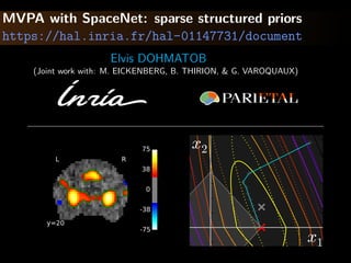
1. MVPA with SpaceNet: sparse structured priors
https://hal.inria.fr/hal-01147731/document
Elvis DOHMATOB
(Joint work with: M. EICKENBERG, B. THIRION, & G. VAROQUAUX)
L R
y=20
-75
-38
0
38
75 x2
x1

2. 1 Introducing the model
2

3. 1 Brain decoding
We are given:
n = # scans; p = number of voxels in mask
design matrix: X ∈ Rn×p
(brain images)
response vector: y ∈ Rn
(external covariates)
Need to predict y on new data.
Linear model assumption: y ≈ X w
We seek to estimate the weights map, w that
ensures best prediction / classification scores
3

4. 1 The need for regularization
ill-posed problem: high-dimensional (n p)
Typically n ∼ 10 − 103
and p ∼ 104
− 106
We need regularization to reduce dimensions and
encode practioner’s priors on the weights w
4

5. 1 Why spatial priors ?
3D spatial gradient (a linear operator)
: w ∈ Rp
−→ ( x w, y w, zw) ∈ Rp×3
penalize image grad w
⇒ regions
Such priors are reasonable
since brain activity is
spatially correlated
more stable maps and more
predictive than unstructured
priors (e.g SVM)
[Hebiri 2011, Michel 2011,
Baldassare 2012, Grosenick 2013,
Gramfort 2013] 5

6. 1 SpaceNet
SpaceNet is a family of “structure + sparsity”
priors for regularizing the models for brain decoding.
SpaceNet generalizes
TV [Michel 2001],
Smooth-Lasso / GraphNet [Hebiri 2011,
Grosenick 2013], and
TV-L1 [Baldassare 2012, Gramfort 2013].
6

7. 2 Methods
7

8. 2 The SpaceNet regularized model
y = X w + “error”
Optimization problem (regularized model):
minimize 1
2 y − Xw 2
2 + penalty(w)
1
2 y − Xw 2
2 is the loss term, and will be different
for squared-loss, logistic loss, ...
8

9. 2 The SpaceNet regularized model
penalty(w) = αΩρ(w), where
Ωρ(w) := ρ w 1 + (1 − ρ)



1
2 w 2
, for GraphNet
w TV , for TV-L1
...
α (0 < α < +∞) is total amount regularization
ρ (0 < ρ ≤ 1) is a mixing constant called the
1-ratio
ρ = 1 for Lasso
9

10. 2 The SpaceNet regularized model
penalty(w) = αΩρ(w), where
Ωρ(w) := ρ w 1 + (1 − ρ)



1
2 w 2
, for GraphNet
w TV , for TV-L1
...
α (0 < α < +∞) is total amount regularization
ρ (0 < ρ ≤ 1) is a mixing constant called the
1-ratio
ρ = 1 for Lasso
Problem is convex, non-smooth, and
heavily-ill-conditioned. 9

11. 2 Interlude: zoom on ISTA-based algorithms
Settings: min f + g; f smooth, g non-smooth
f and g convex, f L-Lipschitz; both f and g
convex
ISTA: O(L f / ) [Daubechies 2004]
Step 1: Gradient descent on f
Step 2: Proximal operator of g
FISTA: O(L f /
√
) [Beck Teboulle 2009]
= ISTA with a “Nesterov acceleration” trick!
10

12. 2 FISTA: Implementation for TV-L1
1e-3
0.10
1e-3
0.25
1e-3
0.50
1e-3
0.75
1e-3
0.90
1e-2
0.10
1e-2
0.25
1e-2
0.50
1e-2
0.75
1e-2
0.90
1e-1
0.10
1e-1
0.25
1e-1
0.50
1e-1
0.75
1e-1
0.90
102
103
Convergencetimeinseconds
α
1 ratio
[DOHMATOB 2014 (PRNI)]
11

13. 2 FISTA: Implementation for GraphNet
Augment X: ˜X := [X cα,ρ ]T
∈ R(n+3p)×p
⇒ ˜Xz(t)
= Xz(t)
+ cα,ρ (z(t)
)
1. Gradient descent step (datafit term):
w(t+1)
← z(t)
− γ˜XT
(˜Xz(t)
− y)
2. Prox step (penalty term):
w(t+1)
← softαργ(w(t+1)
)
3. Nesterov acceleration:
z(t+1)
← (1 + θ(t)
)w(t+1)
− θ(t)
w(t)
Bottleneck: ∼ 80% of runtime spent doing Xz(t)
!
We badly need speedup!
12

14. 2 Speedup via univariate screening
Whereby we detect and remove irrelevant
voxels before optimization problem is even entered!
13

15. 2 XT
y maps: relevant voxels stick-out
L R
y=20
100% brain vol
14

16. 2 XT
y maps: relevant voxels stick-out
L R
y=20
100% brain vol
L R
y=20
50% brain vol
14

17. 2 XT
y maps: relevant voxels stick-out
L R
y=20
100% brain vol
L R
y=20
50% brain vol
L R
y=20
-75
-38
0
38
75
20% brain vol
14

18. 2 XT
y maps: relevant voxels stick-out
L R
y=20
100% brain vol
L R
y=20
50% brain vol
L R
y=20
-75
-38
0
38
75
20% brain vol
The 20% mask has the 3 bright blobs we would
expect to get
... but contains much less voxels ⇒ less run-time
14

19. 2 Our screening heuristic
tp := pth percentile of the vector |XT
y|.
Discard jth voxel if |XT
j y| < tp
L R
y=20
k = 100% voxels
L R
y=20
k = 50% voxels
L R
y=20
-75
-38
0
38
75
k = 20% voxels
Marginal screening [Lee 2014], but without the
(invertibility) restriction k ≤ min(n, p).
The regularization will do the rest... 15

20. 2 Our screening heuristic
See [DOHMATOB 2015 (PRNI)] for a more
detailed exposition of speedup heuristics developed.
16

21. 2 Automatic model selection via cross-validation
regularization parameters:
0 < αL < ... < α3 < α2 < α1 = αmax
mixing constants:
0 < ρM < ... < ρ3 < ρ2 < ρ1 ≤ 1
Thus L × M grid to search over for best
parameters
(α1, ρ1) (α1, ρ2) (α1, ρ3) ... (α1, ρM)
(α2, ρ1) (α2, ρ2) (α2, ρ3) ... (α2, ρM)
(α3, ρ1) (α3, ρ2) (α3, ρ3) ... (α3, ρM)
... ... ... ... ...
(αL, ρ1) (αL, ρ2) (αL, ρL) ... (αL, ρM)
17

22. 2 Automatic model selection via cross-validation
The final model uses average of the the per-fold
best weights maps (bagging)
This bagging strategy ensures more stable and
robust weights maps
18

23. 3 Some experimental results
19

24. 3 Weights: SpaceNet versus SVM
Faces vs objects classification on [Haxby 2001]
Smooth-Lasso weights TV-L1 weights
SVM weights 20

25. 3 Classification scores: SpaceNet versus SVM
21

26. 3 Concluding remarks
SpaceNet enforces both sparsity and structure,
leading to better prediction / classification scores
and more interpretable brain maps.
The code runs in ∼ 15 minutes for “simple”
datasets, and ∼ 30 minutes for very difficult
datasets.
22

27. 3 Concluding remarks
SpaceNet enforces both sparsity and structure,
leading to better prediction / classification scores
and more interpretable brain maps.
The code runs in ∼ 15 minutes for “simple”
datasets, and ∼ 30 minutes for very difficult
datasets.
In the next release, SpaceNet will feature as part
of Nilearn [Abraham et al. 2014]
http://nilearn.github.io.
22

28. 3 Why XT
y maps give a good relevance measure ?
In an orthogonal design, least-squares solution is
ˆwLS = (XT
X)−1
XT
y = (I)−1
XT
y = XT
y
⇒ (intuition) XT
y bears some info on optimal
solution even for general X
23

29. 3 Why XT
y maps give a good relevance measure ?
In an orthogonal design, least-squares solution is
ˆwLS = (XT
X)−1
XT
y = (I)−1
XT
y = XT
y
⇒ (intuition) XT
y bears some info on optimal
solution even for general X
Marginal screening: Set S = indices of top k
voxels j in terms of |XT
j y| values
In [Lee 2014], k ≤ min(n, p), so that
ˆwLS ∼ (XT
S XS)−1
XT
S y
We don’t require invertibility condition
k ≤ min(n, p). Our spatial regularization will do
the rest!
23

30. 3 Why XT
y maps give a good relevance measure ?
In an orthogonal design, least-squares solution is
ˆwLS = (XT
X)−1
XT
y = (I)−1
XT
y = XT
y
⇒ (intuition) XT
y bears some info on optimal
solution even for general X
Marginal screening: Set S = indices of top k
voxels j in terms of |XT
j y| values
In [Lee 2014], k ≤ min(n, p), so that
ˆwLS ∼ (XT
S XS)−1
XT
S y
We don’t require invertibility condition
k ≤ min(n, p). Our spatial regularization will do
the rest!
Lots of screening rules out there: [El Ghaoui
2010, Liu 2014, Wang 2015, Tibshirani 2010,
Fercoq 2015] 23