
Recommandé
Contenu connexe
Tendances
Tendances (20)
Similaire à Stochastic Processes - part 3
Similaire à Stochastic Processes - part 3 (20)
Dernier
Dernier (20)
Stochastic Processes - part 3
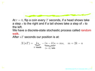
- 1. At t = 0, flip a coin every T seconds, if a head shows take a step s to the right and if a tail shows take a step of s to the left. We have a discrete-state stochastic process called random walk. After nT seconds our position is at: X(nT) = ks |{z} k heads − (n − k)s | {z } (n−k) tails = ms, m = 2k − n AKU-EE/Stochastic/HA, 1st Semester, 85-86 – p.1/134
- 2. P{X(nT) = ms} = n k 0.5k 0.5n−k , m = 2k − n If xi is the ith step E{xi} = s/2 − s/2 = 0, E{x2 i } = s2 /2 + (−s)2 /2 = s2 E{X(nT)} = E{x1 + x2 + · · · + xn} = 0, E{x2 (nT)} = ns2 AKU-EE/Stochastic/HA, 1st Semester, 85-86 – p.2/134
- 3. For large t: P{X(nT) = ms} = n k 0.5k 0.5n−k ∼ exp −(k−np)2 2npq √ 2πnpq For p = q = 0.5, this approximation is valid for − √ npq 6 k − np 6 √ npq ⇒ − √ n 2 6 m − n 2 6 √ n 2 AKU-EE/Stochastic/HA, 1st Semester, 85-86 – p.3/134
- 4. Then the Gaussian approximation converts to: P{X(nT) = ms} = exp − ( (m+n) 2 −n/2)2 2n/4 p 2πn/4 = e−m2/2n pnπ 2 Independent increments: n1 n2 6 n3 n4 ⇒ X(n4T) − X(n3T) is independent of X(n2T) − X(n1T) AKU-EE/Stochastic/HA, 1st Semester, 85-86 – p.4/134
- 5. Wiener Process The limiting form of random walk as T → 0 and n → ∞ is the Wiener process: W(t) = lim T→0 n→∞ X(t) For random walk we had: E{x2 (t = nT)} = ns2 = t T s2 For a meaningful Wiener process we must have: s2 = αT, i.e., s → 0 ⇔ √ T → 0 AKU-EE/Stochastic/HA, 1st Semester, 85-86 – p.5/134
- 6. For random walk: P{X(nT) = ms} = n k pk qn−k = e−m2/2n pnπ 2 The Wiener step: w = ms m √ n = w/s p t/T = w √ t √ T s = w αt AKU-EE/Stochastic/HA, 1st Semester, 85-86 – p.6/134
- 7. Then the 1st order PDF for the Wiener process is: f(w; t) = 1 σ √ 2π exp − w2 2σ2 The variance of a random walk is npq = n/4, and the std.dev= √ n/2 AKU-EE/Stochastic/HA, 1st Semester, 85-86 – p.7/134
- 8. The ACF for a Wiener process: RWW (t1, t2) = E{W(t1)W ∗ (t2)} Because of independent increment property: E{[W(t2) − W(t1)] ∗ W(t1)} = 0 E{W ∗ (t2)W(t1) − |W(t1)|2 } = RWW (t1, t2) − αt1 = 0, t1 t2 ⇒ RWW (t1, t2) = αt1, t1 t2 αt2, t1 t2 The Wiener process is a non-stationary process. AKU-EE/Stochastic/HA, 1st Semester, 85-86 – p.8/134
- 9. Poisson process P{N(t1, t2) = k} = e−λt (λt)k k! , λ = n T For non-overlapping intervals (t1, t2), (t3, t4) then RVs N(t1, t2) and N(t3, t4) are independent E{N(t)} = λt E {N(t1) [N(t2) − N(t1)]} = E{N(t1)}E{N(t2) − N(t1)} = λt1 · λ(t2 − t1) AKU-EE/Stochastic/HA, 1st Semester, 85-86 – p.9/134
- 10. E N2 (t) = λt + (λt)2 ACF: RNN (t1, t2) = λt1 + λ2 t1t2, t1 t2 λt2 + λ2 t1t2, t1 t2 The Poisson process is a non-stationary process. AKU-EE/Stochastic/HA, 1st Semester, 85-86 – p.10/134
- 11. x are called Poisson points. N(t) t x x x x Figure 1: Poisson process AKU-EE/Stochastic/HA, 1st Semester, 85-86 – p.11/134
- 12. Telegraph signal We form a process X(t), using the Poisson points, such that X(t) = 1 if the number of points in (0, t) is even and X(t) = −1 if the number of points in (0, t) is odd. AKU-EE/Stochastic/HA, 1st Semester, 85-86 – p.12/134
- 13. X(t) t - - -1 1 Figure 2: Telegraph signal AKU-EE/Stochastic/HA, 1st Semester, 85-86 – p.13/134
- 14. 1st order PDF: P{X(t) = 1} = e−λt cosh λt P{X(t) = −1} = e−λt sinh λt AKU-EE/Stochastic/HA, 1st Semester, 85-86 – p.14/134
- 15. 2nd order PDF: P{X(t1) = 1, X(t2) = 1} = e−λt2 cosh λt2e−λτ cosh λτ P{X(t1) = 1, X(t2) = −1} = e−λt2 sinh λt2e−λτ sinh λτ P{X(t1) = −1, X(t2) = 1} = e−λt2 cosh λt2e−λτ sinh λτ P{X(t1) = −1, X(t2) = −1} = e−λt2 sinh λt2e−λτ cosh λτ where t2 t1 and τ = t2 − t1 AKU-EE/Stochastic/HA, 1st Semester, 85-86 – p.15/134
- 16. A review: For every stochastic process we have X i,j aia∗ j R(t1, t2) 0, ∀~ a This is the positive (semi)-definite property. And vice-verse, given a positive (semi)-definite function R(t1, t2) we can find a stochastic process with ACF R(t1, t2). AKU-EE/Stochastic/HA, 1st Semester, 85-86 – p.16/134
- 17. Autocovariance function: C(t1, t2) = R(t1, t2) − η(t1)η ∗ (t2) Correlation coefficient: r(t1, t2) = C(t1, t2) p C(t1, t1)C(t2, t2) , |r(t1, t2)| 6 1 Cross-correlation function: RXY (t1, t2) = E{X(t1)Y ∗ (t2)} = R ∗ Y X(t2, t1) AKU-EE/Stochastic/HA, 1st Semester, 85-86 – p.17/134
- 18. Cross- covariance function: CXY (t1, t2) = RXY (t1, t2) − ηX(t1)η ∗ Y (t2) Orthogonal processes: RXY (t1, t2) = 0, ∀t1, t2 Uncorrelated processes: CXY (t1, t2) = 0, ∀t1, t2 AKU-EE/Stochastic/HA, 1st Semester, 85-86 – p.18/134
- 19. a-dependent process: If for a process C(t1, t2) = 0 for |t1 − t2| a correlation a-dependent process: If for a process R(t1, t2) = 0 for |t1 − t2| a White noise process: If the value of a process are uncorrelated for every ti, tj, j 6= i ⇒ C(ti, tj) = 0, i 6= j or C(ti, tj) = q(ti)δ(ti − tj), q(·) 0 AKU-EE/Stochastic/HA, 1st Semester, 85-86 – p.19/134
- 20. A process X(t) is normal if RV {X(t1), · · · , X(tn)} are jointly normal for every n, and {t1, · · · , tn}. The only statistics required are: E{X(t)} = η(t), E{X(ti)X(tj)} = R(ti, tj) f(X(t1), · · · , X(tn)) = exp −0.5X̄C−1 X̄T p (2π)n∆ where X̄ = ~ X − ~ η(t) and Cij = E{X(ti)X(tj)} − η(ti)η(tj) AKU-EE/Stochastic/HA, 1st Semester, 85-86 – p.20/134
- 21. A point process is a set of random points ti on the time axis. The sequence Z1 = t1, Z2 = t2 − t1, · · · , Zn = tn − tn−1 is called a renewal process AKU-EE/Stochastic/HA, 1st Semester, 85-86 – p.21/134
- 22. If X(t) is a WS cyclostationary process, then the shifted process X̄(t) = X(t − θ), θ ∼ Unif(0, T) is WSS. Mean : η̄ = 1 T R T 0 η(t) dt ACF : R̄(τ) = 1 T R T 0 R(t + τ, t) dt Proof: Note: Mean ACF are periodic⇒ E{X(t − θ)} = E{E{X(t − θ)}|θ} = E{ due to cyclo. z }| { η(t − θ) } = 1 T Z T 0 η(t − θ)dθ AKU-EE/Stochastic/HA, 1st Semester, 85-86 – p.22/134
- 23. E{E{X(t + τ − θ)X(t − θ)}|θ} = E{R(t + τ − θ, t − θ)} = 1 T Z T 0 R(t + τ − θ, t − θ)dθ = 1 T Z T 0 R(t1 + τ, t1)dt1 AKU-EE/Stochastic/HA, 1st Semester, 85-86 – p.23/134
- 24. Differentiator: L{X(t)} = X′ (t), ηX′ (t) = η′ X(t), RXX′ (t1, t2) = ∂RXX(t1, t2) ∂t2 because E{X(t1)X′ (t2)} = E{X(t1) d dt2 X(t2)} = ∂ ∂t2 E{X(t1)X(t2)} RX′X′ (t1, t2) = ∂ ∂t1 RXX(t1, t2) = ∂2 ∂t1∂t2 RXX(t1, t2) An integrator follows the same rule. AKU-EE/Stochastic/HA, 1st Semester, 85-86 – p.24/134
- 25. Linear constant coefficient differential equation: n X k=0 akY (k) (t) = X(t), X(k) (0) = 0, k = 0, 1, · · · , n − 1 E ( n X k=0 akY (k) (t) ) = E{X(t)} n X k=0 akη (k) Y (t) = ηX(t), E Y (k) (t) = dk dtk E{Y (t)} η (k) X (0) = 0, k = 0, 1, · · · , n − 1 AKU-EE/Stochastic/HA, 1st Semester, 85-86 – p.25/134
- 26. X(t1) n X k=0 akY (k) (t2) = X(t1)X(t2) E ( X(t1) n X k=0 akY (k) (t2) ) = E{X(t1)X(t2)} n X k=0 akE{X(t1)Y (k) (t2)} = RXX(t1, t2) n X k=0 ak ∂k ∂tk 2 RXY (t1, t2) = RXX(t1, t2), R (k|n−1 0 ) XY (t1, 0) = 0 AKU-EE/Stochastic/HA, 1st Semester, 85-86 – p.26/134
- 27. Y (t2) n X k=0 akY (k) (t1) = X(t1)Y (t2) n X k=0 ak ∂k ∂tk 1 RY Y (t1, t2) = RXY (t1, t2), R (k|n−1 0 ) Y Y (0, t2) = 0 initial conditions: X(k) (0) = 0 ⇒ R (k|n−1 0 ) XY (t1, 0) = 0, R (k|n−1 0 ) Y Y (0, t2) = 0 AKU-EE/Stochastic/HA, 1st Semester, 85-86 – p.27/134
- 28. Ergodicity Time averaging can replace ensemble averaging If we have access to a large number of samples a single ensemble suffices to estimate the desired statistics. X̄ ≈ lim T→∞ 1 T Z T/2 −T/2 X(t; ξ) dt This can only be true iff η(t) =constant. AKU-EE/Stochastic/HA, 1st Semester, 85-86 – p.28/134
- 29. Mean-Ergodic processes Given a stochastic process X(t) with E{X(t)} = η ηT = 1 2T Z T −T X(t)dt, ηT = a RV The process is mean-ergodic iff ηT −→ T →∞ η AKU-EE/Stochastic/HA, 1st Semester, 85-86 – p.29/134
- 30. E{ηT } = 1 2T Z T −T E{X(t)}dt = η Var(ηT ) = E{(ηT − η)2 } −→ T →∞ 0 If this holds true then ηT → η AKU-EE/Stochastic/HA, 1st Semester, 85-86 – p.30/134
- 31. A process X(t) is mean-ergodic iff 1 4T2 Z T −T Z T −T CXX(t1, t2)dt1dt2 −→ T →∞ 0 Proof: 1 4T2 Z T −T Z T −T CXX(t1, t2)dt1dt2 = Var(ηT ) AKU-EE/Stochastic/HA, 1st Semester, 85-86 – p.31/134
- 32. If X(t) is WSS then CXX(t1, t2) = CXX(t1 − t2) ⇒ if ω1 = 0, ω2 = 0 ⇒ R ∞ −∞ R ∞ −∞ CXX(τ)u(t1 − T)u(t1 + T)u(t2 − T)u(t2 + T)e−jω1t1−jω2t2 dt1dt2 = SXX(ω) ∗ 2 sin ωT ω · 2 sin ωT ω This is because u(t1 − T)u(t1 + T)u(t2 − T)u(t2 + T) are separable kernels. F−1 2 sin ωT ω · 2 sin ωT ω = 2T − |τ| AKU-EE/Stochastic/HA, 1st Semester, 85-86 – p.32/134
- 33. Hence, the Mean-Ergodicity condition for WSS process is: 1 2T Z 2T −2T CXX(τ) 1 − |τ| 2T dτ −→ T →∞ 0 AKU-EE/Stochastic/HA, 1st Semester, 85-86 – p.33/134
- 34. Correlation-Ergodic processes A process X(t) is correlation ergodic if Zλ(t) = X(t)X(t + λ) is mean-ergodic. X(t) is correlation-ergodic iff Zλ(t) is mean-ergodic for all λ. RT = 1 2T Z T −T X(t)X(t + λ)dt −→ T →∞ RXX(λ) AKU-EE/Stochastic/HA, 1st Semester, 85-86 – p.34/134
- 35. RZZ(τ) = E{Zλ(t + τ)Zλ(t)} CZZ(τ) = RZZ(τ) − (E{Z(λ)})2 , E{Z(λ)} = RXX(λ) Satisfies 1 2T Z 2T −2T CZZ(τ) 1 − |τ| 2T dτ −→ T →∞ 0 AKU-EE/Stochastic/HA, 1st Semester, 85-86 – p.35/134
- 36. For a deterministic signal X(t), the spectrum is well defined: If represents its Fourier transform, X(ω) = Z +∞ −∞ X(t)e−jωt dt, then |X(ω)|2 represents its energy spectrum. This follows from Parseval’s theorem since the signal energy is given by Z +∞ −∞ x2 (t)dt = 1 2π Z +∞ −∞ |X(ω)|2 dω = E. AKU-EE/Stochastic/HA, 1st Semester, 85-86 – p.36/134
- 37. Thus |X(ω)|2 ∆ω represents the signal energy in the band (ω, ω + ∆ω). However for stochastic processes, a direct application of Fourier transform generates a sequence of random vari- ables for every ω. Moreover, for a stochastic process, E{|X(t)|2 } represents the ensemble average power (instan- taneous energy) at the instant t. AKU-EE/Stochastic/HA, 1st Semester, 85-86 – p.37/134
- 38. To obtain the spectral distribution of power versus frequency for stochastic processes, it is best to avoid infinite intervals to begin with, and start with a finite interval (T, T) XT (ω) = Z T −T X(t)e−jωt dt |XT (ω)|2 2T = 1 2T
- 46. 2 AKU-EE/Stochastic/HA, 1st Semester, 85-86 – p.38/134
- 47. The above equation represents the power distribution as- sociated with that realization based on (T, T). Notice the above equation represents a random variable for every ω and its ensemble average gives, the average power distri- bution based on (T, T). AKU-EE/Stochastic/HA, 1st Semester, 85-86 – p.39/134
- 48. Thus PT (ω)=E |XT (ω)|2 2T = 1 2T Z T −T Z T −T E{X(t1)X∗ (t2)}e−jω(t1−t2) dt1dt2 = 1 2T Z T −T Z T −T RXX(t1, t2)e−jω(t1−t2) dt1dt2 AKU-EE/Stochastic/HA, 1st Semester, 85-86 – p.40/134
- 49. Thus if X(t) is assumed to be WSS then RXX(t1, t2) = RXX(t1 − t2), we have PT (ω) = 1 2T Z T −T Z T −T RXX(t1 − t2)e−jω(t1−t2) dt1dt2. AKU-EE/Stochastic/HA, 1st Semester, 85-86 – p.41/134
- 50. PT (ω) = 1 2T Z 2T −2T RXX(τ)e−jωτ (2T − |τ|)dτ = Z 2T −2T RXX(τ)e−jωτ (1 − |τ| 2T )dτ ≥ 0 Finally letting T → ∞ SXX(ω) = lim T→∞ PT (ω) = Z +∞ −∞ RXX(τ)e−jωτ dτ ≥ 0 RXX(ω) F.T. ←→ SXX(ω) ≥ 0. AKU-EE/Stochastic/HA, 1st Semester, 85-86 – p.42/134
- 51. Wiener-Khinchin theorem: RXX(τ) = 1 2π Z +∞ −∞ SXX(ω)ejωτ dω 1 2π Z +∞ −∞ SXX(ω)dω = RXX(0) = E{|X(t)|2 } = P, the total power. AKU-EE/Stochastic/HA, 1st Semester, 85-86 – p.43/134
- 52. The nonnegative-definiteness property of the ACF translates into the “nonnegative” property for power spectrum, since n X i=1 n X j=1 aia∗ j RXX(ti − tj) = n X i=1 n X j=1 aia∗ j 1 2π Z +∞ −∞ SXX(ω)ejω(ti−tj) dω = 1 2π Z +∞ −∞ SXX(ω)
- 57. n X i=1 aiejωti
- 62. 2 dω ≥ 0. AKU-EE/Stochastic/HA, 1st Semester, 85-86 – p.44/134
- 63. RXX(τ) nonnegative - definite ⇔ SXX(ω) ≥ 0. If X(t) is a real WSS process, then RXX(τ) = RXX(−τ) so that SXX(ω) = Z +∞ −∞ RXX(τ)e−jωτ dτ = Z +∞ −∞ RXX(τ) cos ωτdτ = 2 Z ∞ 0 RXX(τ) cos ωτdτ = SXX(−ω) ≥ 0 AKU-EE/Stochastic/HA, 1st Semester, 85-86 – p.45/134
- 64. If a WSS process X(t) with autocorrelation function RXX(τ) is applied to a linear system with impulse response h(t), then the cross correlation function RXY (τ) and the output autocorrelation function RY Y (τ) are RXY (τ) = RXX(τ) ∗ h∗ (−τ), RY Y (τ) = RXX(τ) ∗ h∗ (−τ) ∗ h(τ). SXY (ω) = F{RXX(ω) ∗ h∗ (−τ)} = SXX(ω)H∗ (ω) AKU-EE/Stochastic/HA, 1st Semester, 85-86 – p.46/134
- 65. SY Y (ω) = F{RY Y (τ)} = SXY (ω)H(ω) = SXX(ω)|H(ω)|2 . AKU-EE/Stochastic/HA, 1st Semester, 85-86 – p.47/134
- 66. The cross spectrum need not be real or nonnegative; How- ever the output power spectrum is real and nonnegative and is related to the input spectrum and the system transfer function as in. The above equations can be used for system identification as well. AKU-EE/Stochastic/HA, 1st Semester, 85-86 – p.48/134
- 67. WSS White Noise Process: If W(t) is a WSS white noise process RWW (τ) = qδ(τ) ⇒ SWW (ω) = q. Thus the spectrum of a white noise process is flat, thus jus- tifying its name. Notice that a white noise process is unre- alizable since its total power is indeterminate. AKU-EE/Stochastic/HA, 1st Semester, 85-86 – p.49/134
- 68. If the input to an unknown system is a white noise process, then the output spectrum is given by SY Y (ω) = q|H(ω)|2 AKU-EE/Stochastic/HA, 1st Semester, 85-86 – p.50/134
- 69. Note that the output spectrum captures the amplitude of transfer function of system characteristics entirely, and for rational systems may be used to determine the pole/zero locations of the underlying system. AKU-EE/Stochastic/HA, 1st Semester, 85-86 – p.51/134
- 70. A WSS white noise process W(t) is passed through a low pass filter (LPF) with bandwidth B/2. The autocorrelation function of the output process is determined as follows: SXX(ω) = q|H(ω)|2 = q, |ω| ≤ B/2 0, |ω| B/2 . AKU-EE/Stochastic/HA, 1st Semester, 85-86 – p.52/134
- 71. RXX(τ) = Z B/2 −B/2 SXX(ω)ejωτ dω = q Z B/2 −B/2 ejωτ dω = qB sin(Bτ/2) (Bτ/2) = qBsinc(Bτ/2) AKU-EE/Stochastic/HA, 1st Semester, 85-86 – p.53/134
- 72. smoothing: Y (t) = 1 2T Z t+T t−T X(τ)dτ represent a “smoothing” operation using a moving window on the input process X(t). The spectrum of the output Y (t) in term of that of X(t) is determined as follows: Y (t) = Z +∞ −∞ h(t − τ)X(τ)dτ = h(t) ∗ X(t) AKU-EE/Stochastic/HA, 1st Semester, 85-86 – p.54/134
- 73. where h(t) = (1/2T)[u(t + T) − u(t − T)]. SY Y (ω) = SXX(ω)|H(ω)|2 . H(ω) = Z +T −T 1 2T e−jωt dt = sinc(ωT) SY Y (ω) = SXX(ω)sinc2 (ωT). AKU-EE/Stochastic/HA, 1st Semester, 85-86 – p.55/134
- 74. Note that the effect of the smoothing operation is to sup- press the high frequency components in the input and the equivalent linear system acts as a low-pass filter (continuous- time moving average) with bandwidth 2π/T in this case, because the first zero of sinc(·) is at π/T AKU-EE/Stochastic/HA, 1st Semester, 85-86 – p.56/134
- 75. Discrete-Time Processes For discrete-time WSS stochastic processes X(nT) with autocorrelation sequence {rk}
- 77. ∞ −∞ or formally defining a continuous time process X(t) = X n X(nT)δ(t − nT), AKU-EE/Stochastic/HA, 1st Semester, 85-86 – p.57/134
- 78. we get the corresponding autocorrelation function to be RXX(τ) = +∞ X k=−∞ rkδ(τ − kT). SXX(ω) = +∞ X k=−∞ rke−jωT ≥ 0, SXX(ω) = SXX(ω + 2π/T) AKU-EE/Stochastic/HA, 1st Semester, 85-86 – p.58/134
- 79. so that SXX(ω) is a periodic function with period 2B = 2π T This gives the inverse relation rk = 1 2B Z B −B SXX(ω)ejkωT dω AKU-EE/Stochastic/HA, 1st Semester, 85-86 – p.59/134
- 80. r0 = E{|X(nT)|2 } = 1 2B Z B −B SXX(ω)dω represents the total power of the discrete-time process X(nT). AKU-EE/Stochastic/HA, 1st Semester, 85-86 – p.60/134
- 81. SXY (ω) = SXX(ω)H∗ (ejω ) SY Y (ω) = SXX(ω)|H(ejω )|2 H(ejω ) = +∞ X n=−∞ h(nT)e−jωnT AKU-EE/Stochastic/HA, 1st Semester, 85-86 – p.61/134
- 82. Matched Filter: Let r(t) represent a deterministic signal s(t) corrupted by noise. Thus r(t) = s(t) + w(t), 0 t t0 where r(t) represents the observed data, and it is passed through a receiver with impulse response h(t). The output y(t) is given by AKU-EE/Stochastic/HA, 1st Semester, 85-86 – p.62/134
- 83. y(t) = ys(t) + n(t) ys(t) = s(t) ∗ h(t), n(t) = w(t) ∗ h(t), and it can be used to make a decision about the presence or absence of s(t) in r(t). AKU-EE/Stochastic/HA, 1st Semester, 85-86 – p.63/134
- 84. Towards this, one approach is to require that the receiver output signal to noise ratio (SNR)0 at time instant t0 be maximized. (SNR)0 = Output signal power at t = t0 Average output noise power = |ys(t0)|2 E{|n(t)|2} = |ys(t0)|2 1 2π R +∞ −∞ Snn(ω)dω =
- 87. 1 2π R +∞ −∞ S(ω)H(ω)ejωt0 dω
- 90. 2 1 2π R +∞ −∞ SW W (ω)|H(ω)|2dω AKU-EE/Stochastic/HA, 1st Semester, 85-86 – p.64/134
- 91. represents the output SNR, and the problem is to maximize (SNR)0 by optimally choosing the receiver filter H(ω). AKU-EE/Stochastic/HA, 1st Semester, 85-86 – p.65/134
- 92. Optimum Receiver for White Noise Input: The simplest input noise model assumes w(t) to be white noise with spectral density N0 (SNR)0 =
- 98. 2 2πN0 R +∞ −∞ |H(ω)|2dω AKU-EE/Stochastic/HA, 1st Semester, 85-86 – p.66/134
- 99. and a direct application of Cauchy-Schwarz’ inequality (SNR)0 ≤ 1 2πN0 Z ∞ −∞ |S(ω)|2 dω = R ∞ 0 s2 (t)dt N0 = Es N0 (1) H(ω) = S∗ (ω)e−jωt0 h(t) = s(t0 − t). (2) The optimum choice for t0 = T. AKU-EE/Stochastic/HA, 1st Semester, 85-86 – p.67/134
- 100. If the receiver is not causal, the optimum causal receiver can be shown to be hopt(t) = s(t0 − t)u(t) and the corresponding maximum (SNR)0 in that case is given by (SNR0) = 1 N0 Z t0 0 s2 (t)dt AKU-EE/Stochastic/HA, 1st Semester, 85-86 – p.68/134
- 101. Optimum Transmit Signal: In practice, the signal s(t) may be the output of a target that has been illuminated by a transmit signal f(t) of finite duration T. In that case s(t) = f(t) ∗ q(t) = Z T 0 f(τ)q(t − τ)dτ, (3) AKU-EE/Stochastic/HA, 1st Semester, 85-86 – p.69/134
- 102. where q(t) represents the target impulse response. One interesting question in this context is to determine the opti- mum transmit signal f(t) with normalized energy that maxi- mizes the receiver output SNR at t = t0. AKU-EE/Stochastic/HA, 1st Semester, 85-86 – p.70/134
- 103. We note that for a given s(t), Eq. (2) represents the op- timum receiver, and (1) gives the corresponding maximum (SNR)0. To maximize (SNR)0 in (1), we may substitute (3) into (1). AKU-EE/Stochastic/HA, 1st Semester, 85-86 – p.71/134
- 104. (SNR)0 = Z ∞ 0
- 108. Z T 0 q(t − τ1)f(τ1)dτ1
- 112. 2 dt = 1 N0 Z T 0 Z T 0 Z ∞ 0 q(t − τ1)q∗ (t − τ2)dt | {z } Ω(τ1,τ2) f(τ2)dτ2f(τ1)dτ1 = 1 N0 Z T 0 Z T 0 Ω(τ1, τ2)f(τ2)dτ2 f(τ1)dτ1 ≤ λmax/N0 Ω(τ1, τ2) = Z ∞ 0 q(t − τ1)q∗ (t − τ2)dt AKU-EE/Stochastic/HA, 1st Semester, 85-86 – p.72/134
- 113. and λmax is the largest eigenvalue of the integral equation Z T 0 Ω(τ1, τ2)f(τ2)dτ2 = λmaxf(τ1), 0 τ1 T. (4) Z T 0 f2 (t)dt = 1. (5) AKU-EE/Stochastic/HA, 1st Semester, 85-86 – p.73/134
- 114. Observe that the kernel Ω(τ1, τ2) captures the target char- acteristics so as to maximize the output SNR at the obser- vation instant, and the optimum transmit signal is the so- lution of the integral equation in (4) subject to the energy constraint in (5). AKU-EE/Stochastic/HA, 1st Semester, 85-86 – p.74/134
- 115. If the noise is not white, one approach is to whiten the input noise first by passing it through a whitening filter, and then proceed with the whitened output as before AKU-EE/Stochastic/HA, 1st Semester, 85-86 – p.75/134
- 116. r(t) = s(t) + w(t) g(t) sg(t) + n(t) Whitening filter w(t) is the colored noise. n(t) is the white noise. AKU-EE/Stochastic/HA, 1st Semester, 85-86 – p.76/134
- 117. Notice that the signal part of the whitened output sg(t) equals sg(t) = s(t) ∗ g(t) AKU-EE/Stochastic/HA, 1st Semester, 85-86 – p.77/134
- 118. Whitening Filter: What is a whitening filter? From the discussion above, the output spectral density of the whitened noise process equals unity, since it represents the normalized white noise by design. 1 = Snn(ω) = SWW (ω)|G(ω)|2 , |G(ω)|2 = 1 SWW (ω) . AKU-EE/Stochastic/HA, 1st Semester, 85-86 – p.78/134
- 119. To be useful in practice, it is desirable to have the whitening filter to be stable and causal as well. Moreover, at times its inverse transfer function also needs to be implementable so that it needs to be stable as well. AKU-EE/Stochastic/HA, 1st Semester, 85-86 – p.79/134
- 120. Any spectral density that satisfies the finite power constraint Z ∞ −∞ SXX(ω)dω ∞ and the Paley-Wiener constraint Z ∞ −∞ | log SXX(ω)| 1 + ω2 dω ∞ can be factorized as SXX(ω) = |H(jω)|2 = H(s)H(−s)|s=jω (6) AKU-EE/Stochastic/HA, 1st Semester, 85-86 – p.80/134
- 121. where H(s) together with its inverse function 1/H(s) rep- resent two filters that are both analytic in ℜ(s) 0. Thus H(s) and its inverse 1/H(s) can be chosen to be stable and causal. Such a filter is known as the Wiener factor, and since has all its poles and zeros in the left half plane, it rep- resents a minimum phase factor. AKU-EE/Stochastic/HA, 1st Semester, 85-86 – p.81/134
- 122. In the rational case, if X(t) represents a real process, then SXX(ω) is even and hence (6) is 0 ≤ SXX(ω2 ) = S̃XX(−s2 )|s=jω = H(s)H(−s)|s=jω. AKU-EE/Stochastic/HA, 1st Semester, 85-86 – p.82/134
- 123. Example: SXX(ω) = (ω2 + 1)(ω2 − 2)2 (ω4 + 1) S̃XX(−s2 ) = (1 − s2 )(2 + s2 )2 1 + s4 . The left half factors are H(s) = (s + 1)(s − √ 2j)(s + √ 2j) s + 1+j √ 2 s + 1−j √ 2 = (s + 1)(s2 + 2) s2 + √ 2s + 1 AKU-EE/Stochastic/HA, 1st Semester, 85-86 – p.83/134
- 124. H(s) represents the Wiener factor for the spectrum SXX(ω). We observe that the poles and zeros (if any) on the jω-axis appear in even multiples in SXX(ω) and hence half of them may be paired with H(s) (and the other half with H(s)) to preserve the factorization condition in (6). Notice that H(s) is stable, and so is its inverse. AKU-EE/Stochastic/HA, 1st Semester, 85-86 – p.84/134
- 125. More generally, if H(s) is minimum phase, then ln H(s) is analytic on the right half plane so that H(ω) = A(ω)e−jϕ(ω) (7) ln H(ω) = ln A(ω) − jϕ(ω) = Z +∞ 0 b(t)e−jωt dt. ln A(ω) = Z t 0 b(t) cos ωtdt ϕ(ω) = Z t 0 b(t) sin ωtdt AKU-EE/Stochastic/HA, 1st Semester, 85-86 – p.85/134
- 126. since cos ωt and sin ωt are Hilbert transform pairs, it follows that the phase function φ(ω) in (7) is given by the Hilbert transform of ln A(ω). Thus ϕ(ω) = H{ln A(ω)}. Eq. (7) may be used to generate the unknown phase func- tion of a minimum phase factor from its magnitude. AKU-EE/Stochastic/HA, 1st Semester, 85-86 – p.86/134
- 127. For discrete-time processes, the factorization conditions take the form Z π −π SXX(ω)dω∞ Z π −π ln SXX(ω)dω − ∞. SXX(ω) = |H(ejω )|2 H(z) = ∞ X k=0 h(k)z−k AKU-EE/Stochastic/HA, 1st Semester, 85-86 – p.87/134
- 128. H(z) is analytic together with its inverse in |z| 1. This unique minimum phase function represents the Wiener fac- tor in the discrete-case. AKU-EE/Stochastic/HA, 1st Semester, 85-86 – p.88/134
- 129. Innovation: A system Γ(s) is called minimum-phase if it is causal, stable and its inverse(1/Γ(s)) is also causal and stable. This means that both Γ(s) and 1/Γ(s) are analytic for ℜ{s} 0 AKU-EE/Stochastic/HA, 1st Semester, 85-86 – p.89/134
- 130. Whitening: Given a stationary process X(t), whitening amounts to finding a minimum-phase system such that its response to X(t) is an orthonormal process I(t). I(t) = Z ∞ −∞ γ(α)X(t − α) dα, RII(τ) = δ(τ) X(t) = Z ∞ −∞ ℓ(β)I(t − β) dβ AKU-EE/Stochastic/HA, 1st Semester, 85-86 – p.90/134
- 131. L(s) = 1 Γ(s) , Γ(s), Whitening filter L(s), Innovation filter SXX(s) = L(s)L(−s) SII(s) | {z } =1 , SXX(ω) = |L(ω)|2 A process X(t) is called regular iff its PSD can be factored as SXX(s) = L(s)L(−s) AKU-EE/Stochastic/HA, 1st Semester, 85-86 – p.91/134
- 132. Rational spectra recursion equations: Y [n] + N X i=1 aiY [n − i] = M X j=0 bjX[n − j] Y (z) X(z) = PM j=0 bjz−j 1 + PN i=1 aiz−i = N(z) D(z) = H(z) AKU-EE/Stochastic/HA, 1st Semester, 85-86 – p.92/134
- 133. Example, continuous process: SXX(ω) = 3 ω4 − ω2 + 1 |s=jω = 3 (s/j)4 − (s/j)2 + 1 s4 + s2 + 1 = 0 ⇒ s2 = −0.5 ± j √ 3 2 = √ 3 s2 + s + 1 | {z } L(s) √ 3 s2 − s + 1 | {z } L(−s) Γ(s) = 1 √ 3 (s2 + s + 1) AKU-EE/Stochastic/HA, 1st Semester, 85-86 – p.93/134
- 134. Example, discrete process: SXX(ω) = 5 − 4 cos ωT 10 − 6 cos ωT ⇒ SXX(z) = 5 − 2(z + z−1 ) 10 − 3(z + z−1) SXX(z) = 2 3 (z − 2)(z − 0.5) (z − 3)(z − 1/3) ⇒ L(z) = r 2 3 z − 0.5 z − 1/3 , 1 Γ(z) = r 2 3 z − 0.5 z − 1/3 AKU-EE/Stochastic/HA, 1st Semester, 85-86 – p.94/134
- 135. Given n RVs {X2, X2, · · · , Xn}, we wish to find n constants {a1, a2, · · · , an} such that we estimate RV S as linear combination Ŝ = n X n=1 anXn = Ê{S|X1, X2, · · · , Xn} MSE criterion: P = E
- 140. S − n X n=1 anXn
- 145. 2 AKU-EE/Stochastic/HA, 1st Semester, 85-86 – p.95/134
- 146. ∂P ∂ai = E 2 ε z }| { S − n X n=1 anXn # (−Xi) = 0 ⇒ ε⊥Xi⇒ε⊥Ŝ z }| { E{εXi} = 0 R11 · · · R1n R21 · · · R2n . . . . . . . . . Rn1 · · · Rnn a1 a2 . . . an = E{SXi}=R0i z }| { R01 R02 . . . R0n , Yule-Walker AKU-EE/Stochastic/HA, 1st Semester, 85-86 – p.96/134
- 147. Vector representation: X = [X1, · · · , Xn], A = [a1, · · · , an], R = E{XT X∗ } Ŝ = AXT = XAT E
- 150. Ŝ
- 153. 2 = E AXT X∗ AT = ARAT AR = R0 ⇒ A = R0R−1 AKU-EE/Stochastic/HA, 1st Semester, 85-86 – p.97/134
- 154. Practical Gramm-Schmidt orthogonalization: Given X = [X1, · · · , Xn] find I = [i1, · · · , in] such that ik is linear combination of X and i1⊥i2⊥ · · · ⊥in ⇒ E{ikim} = δ(k − m) X = IL, L = ℓ1 1 ℓ2 1 · · · ℓn 1 0 ℓ2 2 · · · ℓn 2 0 0 ... . . . 0 0 0 ℓn n IΓ−1 = X ⇔ IL = X AKU-EE/Stochastic/HA, 1st Semester, 85-86 – p.98/134
- 155. E IT I = 1 = E ΓT XT XΓ = = ΓT E XT X Γ ⇒ 1 = ΓT RΓ ⇒ R = ΓT −1 Γ−1 ⇒ AKU-EE/Stochastic/HA, 1st Semester, 85-86 – p.99/134
- 156. R−1 XX = ΓΓT RXX = E XT X = LT E IT I L = LT L RXX = LT L By Cholesky decomposition, we can find the innovation filter L using RXX or the whitening filter Γ using R−1 XX . AKU-EE/Stochastic/HA, 1st Semester, 85-86 – p.100/134
- 157. Stochastic estimate: Estimate the present value of S(t) in terms of another process X(t), the desired estimate Ŝ(t) is an integral of S(t) Ŝ(t) = Ê {S(t)|X(ξ), a 6 ξ 6 b} = Z b a h(α)X(α) dα = n X k=1 h(αk)X(αk)∆α h(α) must be determined. AKU-EE/Stochastic/HA, 1st Semester, 85-86 – p.101/134
- 158. Using orthogonal principle: E ( S(t) − n X k=1 h(αk)X(αk)∆α ! X(ξj) ) ≃ 0, 1 6 j 6 n ⇒ RSX(t, ξj) = n X k=1 h(αk)RXX(αk, ξj)∆α as ∆α → 0 ⇒ RSX(t, ξ) = Z b a h(α)RXX(α, ξ)dα, an integral equation for the unknown h(·). AKU-EE/Stochastic/HA, 1st Semester, 85-86 – p.102/134
- 159. Another derivation: E S(t) − Z b a h(α)X(α)dα X(ξ) ≃ 0, ⇒ RSX(t, ξ) = Z b a h(α)RXX(α, ξ)dα ⇒ Ŝ(t) = Z b a h(α)X(α)dα AKU-EE/Stochastic/HA, 1st Semester, 85-86 – p.103/134
- 160. a t b ⇒ Ŝ(t) is called smoothing t ∋ [a, b] ⇒ Ŝ(t) is called a predictor t a, backward predictor t b, forward predictor (all this is true if X(t) = S(t), no noise.) t ∋ [a, b] X(t) 6= S(t) ⇒ Ŝ(t) is called a filtering operation and a predictor t a, backward filtered-predictor t b, forward filtered-predictor AKU-EE/Stochastic/HA, 1st Semester, 85-86 – p.104/134
- 161. 1) Filtering: Ŝ(t + λ) = Ê{S(t + λ)|S(t)} = aS(t) ⇒ Using orthogonality principle: E{[S(t + λ) − aS(t)]S(t)} = 0 = RSS(λ) − aRSS(0) ⇒ a = RSS(λ) RSS(0) and the variance of estimate, AKU-EE/Stochastic/HA, 1st Semester, 85-86 – p.105/134
- 162. using the fact that E{[S(t + λ) − aS(t)]2 } = E{[S(t + λ) − aS(t)]S(t + λ)} − =0 z }| { E{[S(t + λ) − aS(t)]aS(t)} ⇒ and now the variance is: P = E{[S(t + λ) − aS(t)]S(t + λ)} = RSS(0) − aRSS(λ) aS(t) is an estimate of S(t + λ) in terms of its entire past. AKU-EE/Stochastic/HA, 1st Semester, 85-86 – p.106/134
- 163. Estimate S(t + λ) in terms of S(t) and S′ (t) Ŝ(t + λ) = a1S(t) + a2S′ (t) ⇒ S(t + λ) − Ŝ(t + λ)⊥S(t), S′ (t) ⇒ E{[S(t + λ) − (a1S(t) + a2S′ (t))] S(t)} = 0 E{[S(t + λ) − (a1S(t) + a2S′ (t))] S′ (t)} = 0 AKU-EE/Stochastic/HA, 1st Semester, 85-86 – p.107/134
- 164. E{S(t + λ)S′ (t)} = RSS′ (λ) = −R′ SS(λ) E{S(t)S′ (t)} = −R′ SS(0) E{S(t)S(t)} = −R′′ SS(0), R′ SS(0) = 0 ⇒ Ŝ(t + λ) = S(t) + λS′ (t) AKU-EE/Stochastic/HA, 1st Semester, 85-86 – p.108/134
- 165. 3) Filtering: Ŝ(t) = Ê{S(t)|X(t)} = aX(t) ⇒ Ê{[S(t) − aX(t)]X(t)} = 0 ⇒ a = RSX(0) RXX(0) AKU-EE/Stochastic/HA, 1st Semester, 85-86 – p.109/134
- 166. 4) Interpolation: Ŝ(t + λ) = N X k=−N akS(t + kT), 0 λ T E ( S(t + λ) − N X k=−N akS(t + kT) # S(t + nT) ) = 0, |n| 6 N RSS(λ − nT) = N X k=−N akRSS(KT − nT), |n| 6 N AKU-EE/Stochastic/HA, 1st Semester, 85-86 – p.110/134
- 167. εN (t) = Ŝ(t + λ) − N X k=−N akS(t + kT) var{εN (t)} = E{εN (t)S(t + λ)} = RSS(0) − N X k=−N akRSS(λ − nT) AKU-EE/Stochastic/HA, 1st Semester, 85-86 – p.111/134
- 168. 5) Quadrature: Z = Z b 0 S(t)dt Ẑ = N X n=0 anS(nT), T = T N E Z b 0 S(t)dt − Ẑ S(kT) = 0 ⇒ Z b 0 RSS(t − kT)dt = N X n=0 anRSS(kT − nT), 0 6 k 6 N AKU-EE/Stochastic/HA, 1st Semester, 85-86 – p.112/134
- 169. 6) Smoothing: X(t) = S(t) + ν(t) Ŝ(t) = Ê {S(t)|X(ξ), −∞ ξ ∞} = Z ∞ −∞ h(α)X(t − α)dα Ŝ(t) is the output on a noncausal LTI system with input X(t) S(t) − Ŝ(t)⊥X(ξ), ∀ξ AKU-EE/Stochastic/HA, 1st Semester, 85-86 – p.113/134
- 170. setting ξ = t − τ E S(t) − Z ∞ −∞ h(α)X(t − α)dα X(t − τ) = 0, ∀τ RSX(τ) = Z ∞ −∞ h(α)RXX(τ − α)dα ⇒ SSX(ω) = H(ω)SXX(ω) This is the non-causal Wiener filter. AKU-EE/Stochastic/HA, 1st Semester, 85-86 – p.114/134
- 171. Hilbert transform: H(ω) = −jsgn(ω) = −j, ω 0 j, ω 0 This is called a quadrature filter or phase filter. H{X(t)} = X̌(t) SXX̆(ω) = SXX(ω)(−jsgn(ω))∗ , cross-spectral density SX̆X̆(ω) = SXX(ω) |−jsgn(ω)|2 = SXX(ω) AKU-EE/Stochastic/HA, 1st Semester, 85-86 – p.115/134
- 172. Analytic signals: Z(t) is analytic iff Z(t) = X(t) + jX̆(t) Z(t) is a complex process. F{Z(t)} = X(ω) + j(−jsgn(ω))X(ω) = X(ω) [1 + sgn(ω)] = 2X(ω)U(ω) Hence, the Hilbert transformer is the following ideal causal filter. AKU-EE/Stochastic/HA, 1st Semester, 85-86 – p.116/134
- 173. X(t) 2U(ω) Z(t) Hilbert filter SXZ(ω) = 2SXX(ω)U(ω) SZZ(ω) = 4SXX(ω)U(ω) AKU-EE/Stochastic/HA, 1st Semester, 85-86 – p.117/134
- 174. 2U(ω) = 1 + (−j ∗ j)sgn(ω), F{RXX̆(τ)} = SXX̆(ω) ⇒ RXZ(τ) = RXX(τ) + jR∗ XX̆ (−τ) RZZ(τ) = 2 RXX(τ) + jR∗ XX̆ (−τ) R∗ XX̆ (−τ) = RX̆X(τ) AKU-EE/Stochastic/HA, 1st Semester, 85-86 – p.118/134
- 175. Matched Filter in Colored Noise: r(t) = s(t) + w(t) G(ω) = L−1 (ω) Whitening filter sg(t) + n(t) | {z } h0(t) = sg(t0 − t) t = Matched filter Figure 3: Matched filter for colored noise. AKU-EE/Stochastic/HA, 1st Semester, 85-86 – p.119/134
- 176. L(s)L(−s)|s=jω = |L(jω)|2 = SWW (ω). The optimum receiver is given by h0(t) = sg(t0 − t) sg(t) ↔ Sg(ω) = G(jω)S(ω) = L−1 (jω)S(ω). AKU-EE/Stochastic/HA, 1st Semester, 85-86 – p.120/134
- 177. If we insist on obtaining the receiver transfer function H(ω) for the original colored noise problem we can use the previous figure Fig. 3 H(ω) = L−1 (ω)F{h0(t)} = L−1 (ω)S∗ g (ω)e−jωt0 = L−1 (ω) L−1 (ω)S(ω) ∗ e−jωt0 turns out to be the overall matched filter for the original prob- lem. Once again, transmit signal design can be carried out in this case also. AKU-EE/Stochastic/HA, 1st Semester, 85-86 – p.121/134
- 178. AM/FM Noise Analysis: The noisy AM signal X(t) = m(t) cos(ω0t + θ) + n(t), the noisy FM/PM signal X(t) = A cos(ω0t + ϕ(t) + θ) + n(t), ϕ(t) = c R t 0 m(τ)dτ, FM c m(t), PM. AKU-EE/Stochastic/HA, 1st Semester, 85-86 – p.122/134
- 179. m(t) represents the message signal and θ a random phase jitter in the received signal. In the case of FM ω(t) = ω0 + ϕ′ (t) = ω0 + c m(t), (for PM ω(t) = ω0 + ϕ′ (t) = c m′ (t)), so that the instantaneous frequency for FM is proportional to the message signal. We will assume that both the message process m(t) and the noise process n(t) are WSS with power spectra Smm(ω) and Snn(ω) respectively. We wish to determine whether the AM and FM signals are WSS, and if so their respective power spectral densities. AKU-EE/Stochastic/HA, 1st Semester, 85-86 – p.123/134
- 180. AM signal: if we assume θ ∼ (0, 2π) then RXX(τ) = 1 2 Rmm(τ) cos ω0τ + Rnn(τ) SXX(ω) = SXX(ω − ω0) + SXX(ω + ω0) 2 + Snn(ω). Thus AM represents a stationary process under the above conditions. AKU-EE/Stochastic/HA, 1st Semester, 85-86 – p.124/134
- 181. FM signal: In this case (suppressing the additive noise component) RXX(t + τ/2, t − τ/2) = A2 E{cos(ω0(t + τ/2) + ϕ(t + τ/2) + θ) × cos(ω0(t − τ/2) + ϕ(t − τ/2) + θ)} = A2 2 E{cos[ω0τ + ϕ(t + τ/2) − ϕ(t − τ/2)] + cos[2ω0t + ϕ(t + τ/2) + ϕ(t − τ/2) + 2θ = A2 2 [E{cos(ϕ(t + τ/2) − ϕ(t − τ/2))} cos ω0 −E{sin(ϕ(t + τ/2) − ϕ(t − τ/2))} sin ω0τ] AKU-EE/Stochastic/HA, 1st Semester, 85-86 – p.125/134
- 182. E{cos(2ω0t + ϕ(t + τ/2) + ϕ(t − τ/2) + 2θ)} = E{cos(2ω0t + ϕ(t + τ/2) + ϕ(t − τ/2))}E{cos 2θ} −E{sin(2ω0t + ϕ(t + τ/2) + ϕ(t − τ/2))}E{sin 2θ} = 0. RXX(t + τ/2, t − τ/2) = A2 2 [a(t, τ) cos ω0τ − b(t, τ) sin ω0τ] (8) a(t, τ) = E{cos(ϕ(t + τ/2) − ϕ(t − τ/2))} (9) b(t, τ) = E{sin(ϕ(t + τ/2) − ϕ(t − τ/2))} (10) AKU-EE/Stochastic/HA, 1st Semester, 85-86 – p.126/134
- 183. In general a(t, τ) and b(t, τ) depend on both t and τ so that noisy FM is not WSS in general, even if the message pro- cess m(t) is WSS. AKU-EE/Stochastic/HA, 1st Semester, 85-86 – p.127/134
- 184. In the special case when m(t) is a stationary Gaussian process, ϕ(t) is also a stationary Gaussian process with autocorrelation function Rϕ′ϕ′ (τ) = c2 Rmm(τ) = −d2 Rϕϕ(τ) dτ2 for the FM case. AKU-EE/Stochastic/HA, 1st Semester, 85-86 – p.128/134
- 185. In that case the random variable Y = ϕ(t + τ/2) − ϕ(t − τ/2) ∼ N(0, σ2 Y ) (11) σ2 Y = 2(Rϕϕ(0) − Rϕϕ(τ)). (12) E{ejωY } = e−ω2σ2 Y /2 = e−(Rϕϕ(0)−Rϕϕ(τ))ω2 (13) which for ω = 1 gives E{ejY } = E{cos Y } + jE{sin Y } = a(t, τ) + jb(t, τ), (14) AKU-EE/Stochastic/HA, 1st Semester, 85-86 – p.129/134
- 186. where we have made use of (11) and (9)-(10). On comparing (14) with (13) we get a(t, τ) = e−(Rϕϕ(0)−Rϕϕ(τ)) b(t, τ) ≡ 0 so that the FM autocorrelation function in (8) simplifies into RXX(τ) = A2 2 e−(Rϕϕ(0)−Rϕϕ(τ)) cos ω0τ. (15) AKU-EE/Stochastic/HA, 1st Semester, 85-86 – p.130/134
- 187. Notice that for stationary Gaussian message input m(t) (or φ(t) ), the nonlinear output X(t) is indeed SSS with auto- correlation function as in (15). AKU-EE/Stochastic/HA, 1st Semester, 85-86 – p.131/134
- 188. Narrowband FM: If Rϕϕ(τ) ≪ 1 (15) may be approximated as(ex ≈ 1 − x, |x| ≪ 1) RXX(τ) = A2 2 {(1 − Rϕϕ(0)) + Rϕϕ(τ)} cos ω0τ which is similar to the AM case. Hence narrowband FM and ordinary AM have equivalent performance in terms of noise suppression. AKU-EE/Stochastic/HA, 1st Semester, 85-86 – p.132/134
- 189. Wideband FM: This case corresponds to Rϕϕ(τ) 1 In that case a Taylor series expansion or Rϕϕ(τ) gives Rϕϕ(0) + 1 2 R′′ ϕϕ(0)τ2 + · · · = Rϕϕ(0) − c2 2 Rmm(0)τ2 + · · · and substituting this into (15) we get RXX(τ) = A2 2 e− c2 2 Rmm(0)τ2+··· cos ω0τ AKU-EE/Stochastic/HA, 1st Semester, 85-86 – p.133/134
- 190. so that the power spectrum of FM in this case is given by SXX(ω) = 1 2 {S(ω − ω0) + S(ω + ω0)} S(ω) ≈ A2 2 e−ω2/2c2Rmm(0) . Notice that SXX(ω) always occupies infinite bandwidth irrespective of the actual message bandwidth and this capacity to spread the message signal across the entire spectral band helps to reduce the noise effect in any band. AKU-EE/Stochastic/HA, 1st Semester, 85-86 – p.134/134