Stochastic Processes - part 5

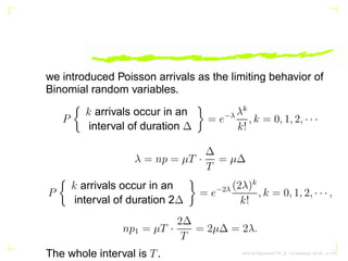
we introduced Poisson arrivals as the limiting behavior of
Binomial random variables.
P

k arrivals occur in an
interval of duration ∆

= e−λ λk
k!
, k = 0, 1, 2, · · ·
λ = np = µT ·
∆
T
= µ∆
P

k arrivals occur in an
interval of duration 2∆

= e−2λ (2λ)k
k!
, k = 0, 1, 2, · · · ,
np1 = µT ·
2∆
T
= 2µ∆ = 2λ.
The whole interval is T. AKU-EE/Stochastic/HA, 1st Semester, 85-86 – p.1/63

Poisson arrivals over an interval form a Poisson random
variable whose parameter depends on the duration of that
interval. Moreover because of the Bernoulli nature of the
underlying basic random arrivals, events over nonoverlap-
ping intervals are independent.
AKU-EE/Stochastic/HA, 1st Semester, 85-86 – p.2/63

We shall use these two key observations to define a
Poisson process formally. X(t) = n(0, t) represents a
Poisson process if (i) the number of arrivals n(t1, t2) in an
interval (t1, t2) of length t = t2 − t1 is a Poisson random
variable with parameter λt
P{n(t1, t2) = k} = e−λt (λt)k
k!
, k = 0, 1, 2, · · · , t = t2 − t1

If the intervals (t1, t2) and (t3, t4) are nonoverlapping, then
the random variables n(t1, t2) and n(t3, t4) are independent.

Since n(0, t) = P(λt)
E[X(t)] = E[n(0, t)] = λt
E[X2
(t)] = E[n2
(0, t)] = λt + λ2
t2
.
RXX(t1, t2) = λ2
t1t2 + λmin(t1, t2).

the Poisson process X(t) does not represent a WSS pro-
cess.

Define a binary level process
Y (t) = (−1)X(t)
that represents a telegraph signal. Notice that the
transition instants {ti} are random. Although X(t) does not
represent a WSS process, its derivative X′
(t) does
represent a WSS process.

µX′ (t) =
dµX(t)
dt
=
dλt
dt
= λ, a constant
RXX′ (t1, t2) = ∂RXX (t1,t2)
∂t2
=

λ2
t1t1 ≤ t2
λ2
t1 + λt1 t2
= λ2
t1 + λU(t1 − t2)
RX′X′ (t1, t2) =
∂RXX′ (t1, t2)
∂t1
= λ2
+ λδ(t1 − t2).
it follows that X′
(t) is a WSS process. Thus nonstationary
inputs to linear systems can lead to WSS outputs.

Sum of Poisson Processes:
If X1(t) and X2(t) represent two independent Poisson
processes, then their sum X1(t) + X2(t) is also a Poisson
process with parameter (λ1 + λ2)t.

Random selection of Poisson Points:
Let t1, t2, · · · , ti, · · · represent random arrival points
associated with a Poisson process X(t) with parameter λt
and associated with each arrival point, define an
independent Bernoulli random variable Ni, where
P(Ni = 1) = p, P(Ni = 0) = q = 1 − p.

Y (t) =
X(t)
X
i=1
Ni;Z(t) =
X(t)
X
i=1
(1 − Ni) = X(t) − Y (t) ⇒
both Y (t) and Z(t) are independent Poisson processes with
parameters λpt and λqt respectively

Proof:
Y (t) =
∞
X
n=k
P{Y (t) = k|X(t) = n}P{X(t) = n)}.
But given X(t) = n, we have
Y (t) =
n
X
i=1
Ni ∼ B(n, p)
so that
P{Y (t) = k|X(t) = n} =
n
k

pk
qn−k
, 0 ≤ k ≤ n,

P{X(t) = n} = e−λt (λt)n
n!
.
by substituting, we get
P{Y (t) = k} = e−λt
∞
X
n=k
n!
(n−k)!k!
pk
qn−k (λt)n
n!
=
pk
e−λt
k!
(λt)k
∞
X
n=k
(qλt)n−k
(n−k)!
| {z }
exp(qλt)
= (λpt)k e−(1−q)λt
k!
= e−λpt (λpt)k
k!
, k = 0, 1, 2, · · ·

More generally,
P{Y (t) = k, Z(t) = m} = P{Y (t) = k, X(t) − Y (t) = m}
= P{Y (t) = k, X(t) = k + m}
= P{Y (t) = k|X(t) = k + m}P{X(t) = k + m}
=
k+m
k

pk
qm
· e−λt (λt)k+m
(k + m)!
= e−λpt (λpt)n
k!
| {z }
P (Y (t)=k)
e−λqt (λqt)n
m!
| {z }
P (Z(t)=m)
= P{Y (t) = k}P{Z(t) = m},

Thus random selection of Poisson points preserve the Pois-
son nature of the resulting processes. However, determin-
istic selection from a Poisson process destroys the Poisson
property for the resulting processes.

Inter-arrival Distribution for Poisson Processes
If τ1 is to denote the time interval (delay) to the first arrival
from any fixed point t0.
Fτ1 (t) = P{τ1 ≤ t} = P{X(t) 0} = P{n(t0, t0 + t) 0}
= 1 − P{n(t0, t0 + t) = 0} = 1 − e−λt
fτ1 (t) =
dFτ1 (t)
dt
= λe−λt
, t ≥ 0
τ1 is an exponential random variable with parameter λ so
that E{τ1} = 1/λ

Similarly, let tn represent the nth random arrival point for a
Poisson process.
Ftn (t) = P{tn ≤ t} = P{X(t) ≥ n}
= 1 − P{X(t) n} = 1 −
n−1
X
k=0
(λt)k
k!
e−λt
⇒
ftn (x) =
dFtn (x)
dx
= −
n−1
X
k=1
λ(λx)k−1
(k − 1)!
e−λx
+
n−1
X
k=0
λ(λx)k
k!
e−λx
=
λn
xn−1
(n − 1)!
e−λx
, x ≥ 0

which represents a gamma density function . i.e., the
waiting time to the nth Poisson arrival instant has a gamma
distribution. Moreover
tn =
n
X
i=1
τi
where τi is the random inter-arrival duration between the
(i1)th and ith events.

Hence using their characteristic functions, it follows that all
inter-arrival durations of a Poisson process are
independent exponential random variables with common
parameter λ
fτi
(t) = λe−λt
, t ≥ 0.

Thus if we systematically tag every mth outcome of a
Poisson process X(t) with parameter λt to generate a new
process e(t), then the inter-arrival time between any two
events of e(t) is a gamma random variable.
E[e(t)] = m/λ, and if λ = mµ, then E[e(t)] = 1/µ.
The inter-arrival time of e(t) in that case represents an
Erlang-m random variable, and e(t) an Erlang-m process.

In summary, if Poisson arrivals are randomly redirected to
form new queues, then each such queue generates a new
Poisson process. However if the arrivals are systemati-
cally redirected 1st arrival to 1st counter, 2nd arrival to 2nd
counter, mth to mth , (m + 1)th, then the new subqueues
form Erlang-m processes.

Poisson Departures between Exponential Inter-arrivals
If X(t) ∼ P(λt) and Y (t) ∼ P(µt) represent two indepen-
dent Poisson processes called arrival and departure pro-
cesses.

Z represent the random interval between any two
successive arrivals of X(t). Z has an exponential
distribution with parameter λ Let N represent the number
of “departures” of Y (t) between any two successive
arrivals of X(t). Then from the Poisson nature of the
departures we have
P{N = k|Z = t} = e−µt (µt)k
k!
.

P{N = k} =
Z ∞
0
P{N = k|Z = t}fZ(t)dt
=
Z ∞
0
e−µt (µt)k
k!
λe−λt
dt
=
λ
k!
Z ∞
0
(µt)k
e−(λ+µ)t
dt
=
λ
λ + µ

µ
λ + µ
k
1
k!
Z ∞
0
xk
e−x
dx
| {z }
k!
=

λ
λ + µ

µ
λ + µ
k
, k = 0,

the random variable N has a geometric distribution. Thus
if customers come in and get out according to two indepen-
dent Poisson processes at a counter, then the number of
arrivals between any two departures has a geometric dis-
tribution. Similarly the number of departures between any
two arrivals also represents another geometric distribution.

Suppose a cereal manufacturer inserts a sample of one
type of coupon randomly into each cereal box. Suppose
there are n such distinct types of coupons. One interesting
question is that how many boxes of cereal should one buy
on the average in order to collect at least one coupon of
each kind?

Stopping Times
Let X1(t), X2(t), · · · , Xn(t) represent n independent identi-
cally distributed Poisson processes with common parame-
ter λt Let ti1, ti2, · · · represent the first, second, random ar-
rival instants of the process Xi(t), i = 1, 2, · · ·. They will
correspond to the first, second, appearance of the ith type
coupon in the above problem.

X(t) =
n
X
i=1
Xi(t),
so that the sum X(t) is also a Poisson process with
parameter µt
µ = nλ

1/λ represents The average inter-arrival duration between
any two arrivals of Xi(t), i = 1, 2, · · · whereas 1/µ repre-
sents the average inter-arrival time for the combined sum
process X(t)

the stopping time T to be that random time instant by which
at least one arrival of X1(t), X2(t), · · · , Xn(t) has occurred.
T = max (t11, t21, · · · , ti1, · · · , tn1).

ti1, i = 1, 2, · · · , n are independent exponential random
variables with common parameter λ. This gives
FT (t) = P{T ≤ t} = P{max (t11, t21, · · · , tn1) ≤ t}
= P{t11 ≤ t, t21 ≤ t, · · · , tn1 ≤ t}
= P{t11 ≤ t}P{t21 ≤ t} · · · P{tn1 ≤ t} = [Fti(t)]n
.
FT (t) = (1 − e−λt
)n
, t ≥ 0
represents the probability distribution function of the
stopping time random variable T.

P(T t) = 1 − FT (t) = 1 − (1 − e−λt
)n
, t ≥ 0
To compute its mean
E{T} =
Z ∞
0
P(T t)dt =
Z ∞
0
{1 − (1 − e−λt
)n
}dt.
1 − e−λt
= x,

E{T} =
1
λ
Z 1
0
(1 − xn
)
dx
1 − x
=
1
λ
Z 1
0
1 − xn
1 − x
dx
=
1
λ
Z 1
0
(1 + x + x2
+ · · · + xn−1
)dx =
1
λ
n
X
k=1
xk
k

1
0
E{T} =
1
λ

1 +
1
2
+
1
3
+ · · · +
1
n

≃
1
µ
n(ln n + γ)
where γ ≃ 0.5772157 · · · is the Euler’s constant.

Then we obtain the key relation
T =
N
X
i=1
Yi
E{T|N = n} = E{
n
X
i=1
Yi|N = n} = E{
n
X
i=1
Yi} = nE{Yi}
since {Yi} and N are independent random variables, and
hence
E{T} = E[E{T|N = n}] = E{N}E{Yi}

Because Yi ∼ exp(µ) ⇒ E{Yi} = 1/µ
E{N} ≃ n(ln n + γ).
Thus on the average a customer should buy about n ln n or
slightly more, boxes to guarantee that at least one coupon
of each type has been collected.

Next, consider a slight generalization to the above problem:
What if two kinds of coupons (each of n type) are mixed up,
and the objective is to collect one complete set of coupons
of either kind?

Let Xi(t) and Yi(t), i = 1, 2, · · · represent the two kinds of
coupons (independent Poisson processes) that have been
mixed up to form a single Poisson process Z(t) with
normalized parameter unity.
Z(t) =
n
X
i=1
[Xi(t) + Yi(t)] ∼ P(t).

As before let ti1, ti2, · · · represent the first, second, arrivals of
the process Xi(t), and τi1, τi2, · · · represent the first, second,
arrivals of the process Yi(t), i = 1, 2, · · · , n. The stopping
time T1 in this case represents that random instant at which
either all X - type or all Y - type have occurred at least once

T1 = min{X, Y }
X = max (t11, t21, · · · , tn1)
Y = max (τ11, τ21, · · · , τn1).
the random variables X and Y have the same distribution
with λ replaced by 1/2n (since µ = 1 and there are 2n
independent and identical processes as before), and hence
FX(t) = FY (t) = (1 − e−t/2n
)n
, t ≥ 0.

FT1 (t) = P(T1 ≤ t) = P(min{X, Y } ≤ t)
= 1 − P(min{X, Y } t) = 1 − P(X t, Y t)
= 1 − P(X t)P(Y t)
= 1 − (1 − FX(t))(1 − FY (t))
= 1 − {1 − (1 − e−t/2n
)n
}2
, t ≥ 0
to be the probability distribution function of the new
stopping time T1.

E{T1} =
Z ∞
0
P(T1 t)dt =
Z ∞
0
{1 − FT1 (t)}dt
=
Z ∞
0
{1 − (1 − e−t/2n
)n
}2
dt.
1 − e−t/2n
= x, or 1
2n
e−t/2n
dt = dx, dt = 2ndx
1−x
.

E{T1} = 2n
Z 1
0
(1 − xn
)2 dx
1 − x
= 2n
Z 1
0

1 − xn
1 − x

(1 − xn
)dx
= 2n
Z 1
0
(1 + x + x2
+ · · · + xn−1
)(1 − xn
)dx
= 2n
Z 1
0
(
n−1
X
k=0
xk
−
n−1
X
k=0
xn+k
)dx
= 2n

1 +
1
2
+
1
3
+ · · · +
1
n

−

1
n + 1
+
1
n + 2
+ · · · +
1
2n

= 2n(ln(n/2) + γ).

the total number of random arrivals N up to T1 is related
where Yi ∼Exponential(1),
E{N} = E{T1} ≃ 2n(ln(n/2) + γ).

We can generalize the stopping times in yet another way:
Poisson Quotas:
X(t) =
n
X
i=1
Xi(t) ∼ P(µt)

The stopping time T in this case is that random time
instant at which any r processes have met their quota
requirement where is r 6 n given. The problem is to
determine the probability density function of the stopping
time random variable T, and determine the mean and
variance of the total number of random arrivals N up to the
stopping time T.

Solution:
ti1, ti2, · · · represent the first, second, arrivals of the ith
process Xi(t), and define
Yij = tij − ti,j−1
the inter-arrival times Yjj and independent, exponential
random variables with parameter λi and hence
ti,mi
=
mi
X
j=1
Yij ∼ Gamma(mi, λi)

where Xi(t) are independent, identically distributed Pois-
son processes with common parameter λit, µ = λ1 +
· · · + λn, integers m1, m2, · · · , mn represent the preas-
signed number of arrivals (quotas) required for processes
X1(t), X2(t), · · · , Xn(t) in the sense that when mi arrivals of
the process Xi(t) have occurred, the process Xi(t) satisfies
its quota requirement.

Ti to the stopping time for the ith process; i.e., the
occurrence of the mith arrival equals Ti. Thus
Ti = ti,mi
∼ Gamma(mi, λi), i = 1, 2, · · · , n
fTi
(t) =
tmi−1
(mi − 1)!
λmi
i e−λit
, t ≥ 0.

Since the n processes are independent, the associated
stopping times Ti, i = 1, 2, · · · , n are also independent
random variables, a key observation. Given independent
gamma random variables T1, T2, · · · , Tn we form their order
statistics: This gives
T(1) T(2) · · · T(r) · · · T(n).
The desired stopping time T when r processes have
satisfied their quota requirement is given by the rth order
statistics T(r).
T = T(r)

The density function of the stopping time random variable
T where r types of arrival quota requirements have been
satisfied.
fT (t) =
n!
(r − 1)!(n − r)!
Fk−1
Ti
(t)[1 − FTi
(t)]n−k
fTi
(t)
Integrating by parts from fTi
(t), we have
FTi
(t) = 1 −
mi−1
X
k=0
(λit)k
k!
e−λit
, t 0.

If N represents the total number of all random arrivals up
to T,
T =
N
X
i=1
Yi
where Yi are the inter-arrival intervals for the process X(t),
and hence
E{T} = E{N}E{Yi} = 1
µ
E{N}
with normalized mean value µ = 1 for the sum process
X(t), we get
E{N} = E{T}.

To relate the higher order moments of N and T we can use
their characteristic functions.
E{ejωT
} = E{e
jω
N
P
i=1
Yi
} = E{E[e
jω
n
P
i=1
Yi
|N = n]
| {z }
[E{ejωYi }]n
}
= E[{E{ejωYi
}|N = n}n
].
But Y i ∼Exponential(1) and independent of N so that
E{ejωYi
|N = n} = E{ejωYi
} =
1
1 − jω

E{ejωT
} =
∞
X
n=0
[E{ejωYi
}]n
P(N = n) =E

1
1−jω
N

= E{(1−jω)−N
}
∞
X
k=0
(jω)k
k!
E{Tk
} =
∞
X
k=0
(jω)k
k!
E{N(N + 1) · · · (N + k − 1)}
E{Tk
} = E{N(N + 1) · · · (N + k − 1)},
var{N} = var{T} − E{T}.

In probability theory, a (discrete-time) martingale is a
discrete-time stochastic process (i.e., a sequence of
random variables) X1, X2, X3, · · · that satisfies the identity
E(Xn+1|X1, · · · , Xn) = Xn
i.e., the conditional expected value of the next observation,
given all of the past observations, is equal to the last ob-
servation. As is frequent in probability theory, the term was
adopted from the language of gambling.

Somewhat more generally, a sequence Y1, Y2, Y3, · · · is said
to be a martingale with respect to another sequence
X1, X2, X3, · · · if
E(Yn+1|X1, · · · , Xn) = Yn, ∀n

A continuous-time martingale is a zero-drift stochastic
process. That is, a random variable θ follows a
continuous-time martingale iff
dθ = σdz
where dz is a Wiener process and the variable σ is a
constant or a stochastic process that may depend on θ or
other stochastic variables.

Originally, martingale referred to a class of betting strate-
gies popular in 18th century France. The simplest of these
strategies was designed for a game in which the gambler
wins his stake if a coin comes up heads and loses it if the
coin comes up tails. The strategy had the gambler double
his bet after every loss, so that the first win would recover all
previous losses plus win a profit equal to the original stake.

Since as a gambler’s wealth and available time jointly ap-
proach infinity his probability of eventually flipping heads ap-
proaches 1, the martingale betting strategy was seen as a
sure thing by those who practiced it. Of course in reality the
exponential growth of the bets would quickly bankrupt those
foolish enough to use the martingale after even a moder-
ately long run of bad luck.

The concept of martingale in probability theory was intro-
duced by Paul Pierre Lévy, and much of the original devel-
opment of the theory was done by Joseph Leo Doob. Part
of the motivation for that work was to show the impossibility
of successful betting strategies.

Stochastic Processes - part 5

Recommandé

Recommandé

Contenu connexe

Tendances

Tendances (20)

Similaire à Stochastic Processes - part 5

Similaire à Stochastic Processes - part 5 (20)

Dernier

Dernier (20)

Stochastic Processes - part 5