This month we’re going to get a bit sensitive with a simple feature which allows us to very quickly perform some sensitivity analysis but first we’re going to look at a few tips for finding your way around a large spreadsheet. The features covered here are based on Excel 2003 however most can still be found in other versions. For more information, please contact +61 2 9080 4050, edinfo@iir.com.au , or visit: http://bit.ly/iired

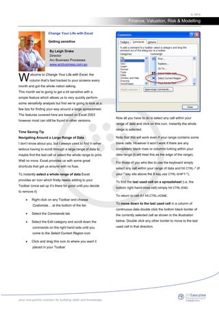
1. E-TIPS
Finance, Valuation, Risk & Modelling
Change Your Life with Excel
Getting sensitive
By Leigh Drake
Director
Arc Business Processes
www.arcbusiness.com.au
W elcome to Change Your Life with Excel, the
column that’s fast tracked to your screens every
month and got the whole nation talking.
This month we’re going to get a bit sensitive with a
simple feature which allows us to very quickly perform
some sensitivity analysis but first we’re going to look at a
few tips for finding your way around a large spreadsheet.
The features covered here are based on Excel 2003
Now all you have to do is select any cell within your
however most can still be found in other versions.
range of data and click on this icon. Instantly the whole
range is selected.
Time Saving Tip
Navigating Around a Large Range of Data Note that this will work even if your range contains some
I don’t know about you, but I always used to find it rather blank cells. However it won’t work if there are any
tedious having to scroll through a large range of data to completely blank rows or columns lurking within your
maybe find the last cell or select the whole range to print. data range (it will treat this as the edge of the range).
Well no more. Excel provides us with some great
For those of you who like to use the keyboard simply
shortcuts that get us around with no fuss.
select any cell within your range of data and hit CTRL-* (if
To instantly select a whole range of data Excel your * key sits above the 8 key use CTRL-SHIFT-*).
provides an icon which firstly needs adding to your
To find the last used cell on a spreadsheet (i.e. the
Toolbar (once set up it’s there for good until you decide
bottom right hand-most cell) simply hit CTRL-END.
to remove it)
To return to cell A1 hit CTRL-HOME.
• Right click on any Toolbar and choose
To move down to the last used cell in a column of
Customize… at the bottom of the list
continuous data double click the bottom black border of
• Select the Commands tab the currently selected cell as shown in the illustration
• Select the Edit category and scroll down the below. Double click any other border to move to the last
commands on the right hand side until you used cell in that direction.
come to the Select Current Region icon
• Click and drag this icon to where you want it
placed in your Toolbar
your one-partner solution for building skills and knowledge

2. E-TIPS
Finance, Valuation, Risk & Modelling
Excel provides a built-in function called PMT (it’s short for
“payment” before you ask). Whilst this month’s column
isn’t really about using specific built-in functions, I’ll go off
on a bit of a tangent and explain how to set this one up
as you may find it useful.
PMT requires the following arguments:
rate = annual interest rate
nper = number of repayment periods
pv = amount of the loan
For ease of use, set out each of these 3 arguments on
separate lines as below and allocate some values to
them.
The keyboard equivalent for this is to hold CTRL and
select the arrow key for whichever direction you require.
Finally, the more obscure keyboard command CTRL-.
(full-stop) selects each successive corner cell in a pre-
selected range.
Secret – The Sensitivity Table
The formula in cell B4 then becomes:
So what’s this bit all about? Well suppose for example
that you have a scenario where you want to see the =PMT(B2/12,B3,B1)
effect of various interest rates on loan repayments or the A couple of things to note with this formula:
effect of various sales prices and volumes on your profit.
• The annual interest rate in B2 has to be divided
It wouldn’t be too difficult to set up a spreadsheet using
by 12 as we have decided our period will be
lots of formulas to do this but why bother when Excel has
months
a way of doing this much faster once you know how (this
column is all about helping reduce your screen time and • The result will be a negative number. By
increasing your play time unless like me the 2 amount to convention Excel shows payments as negative
the same thing!) and receipts as positive. Simply put a minus
sign in front of the function to display the result
This is one of those features in Excel that has probably
as positive
been staring you in the face but you’ve never really
noticed it. Let’s start with the first example above to see Entering this formula in cell B4 gives an answer of
the effect of interest rates on loan repayments. In Excel $198.01.
terminology we will set up a one-variable table since this
Okay, I’m back off my tangent. Now that we have the
only has one variable – interest rates.
base formula set up we can very quickly create our
Firstly we need to set up a single formula (the base sensitivity table.
formula) which derives the repayments on a loan at a
In a nearby blank region, type in the range of interest
certain interest rate.
rates you wish to see the effect of.
your one-partner solution for building skills and knowledge

3. E-TIPS
Finance, Valuation, Risk & Modelling
We now have to tell Excel 2 things:
1. What values we want to show in the body of the
data table, range E6:E14 i.e. the repayment
amounts
2. What the numbers in the range D6:D14
represent i.e. interest rates
• Select OK
The first of these we do by selecting the cell at the top of
the column where our values will appear, cell E5, and You will see that the table is now populated with the
reference the cell in our formula which calculates the monthly repayments on a loan of $10,000 over 60
repayments i.e. cell B4. months for various interest rates.
nd
To tell Excel the 2 piece of information requires our
Excel secret.
• Select the range of the entire table D5:E14
• Select Data | Table… from the Menu Bar
• In the Table input box under Column input cell
reference cell B2 which is where the base
formula records the interest rate (note that if we
were filling values across a row we would use
the Row input cell field)
This will automatically update when you change the loan
amount and/or repayment term in the base formula or
when you change any of the interest rates in column D.
your one-partner solution for building skills and knowledge

4. E-TIPS
Finance, Valuation, Risk & Modelling
The advantages to using this method are: Similar to before, the first of these is done by selecting, in
this case, the top left-most cell C10 and referencing the
• You only need to set up one formula. Using
cell calculating profit in the base formula B6.
more conventional methods would require you
to enter a formula in each of cells E6 to E14. • Select the range of the entire table C10:G15
• Changes can be made very quickly by editing • Select Data | Table… from the Menu Bar
the one base formula
• In the Table input box under Row input cell
nd
If you’re still hanging in there we’ll now look at our 2 reference cell B1 which is where the base
example which looks at the effect on profit of 2 variables formula records the sales price and which is
and which requires a 2-variable table. across the row in our table
As above, we set up a base formula which will derive the • Under Column input cell reference cell B2 which
profit from the variables as below. The formulas used are is where the base formula records the sales
shown next to the cells for your information (you don’t units and which is down the column in our table
need to type these!)
Again, set up the range of variables for both sales price
and sales units as below. In this example, sales prices
are along the top and sales units are down the side.
• Select OK
The table is now populated with the profit resulting from
various combinations of price and units.
We need to tell Excel 3 things:
1. What values we want to show in the body of the
data table, range D11:G15 i.e. the profit Changing the profit % in the base formula or sales price
and/or units in the table will automatically update the
2. What the numbers in the range D10:G10
profit amounts.
represent i.e. sales price
Phew! Once you get the hang of these methods you will
3. What the numbers in the range C11:C15
see that this is much quicker than setting up a
represent i.e. sales units
conventional multi-formula table.
Until next time, happy Excelling.
your one-partner solution for building skills and knowledge