1. Engr. Ayaz Waseem ( Lecturer/Lab Engr., CED) Columns
LECTURE # 6
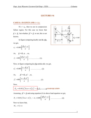
CASE 8: e IS GIVEN AND e < eb:
If e < eb , then we are in compression
failure region. For this case we know that
fs ≠ fy , but whether fs′ = fy or not, this is not
known.
In figure comparing ∆ a b c and ∆ c f g,
we get,





 −
=
a
ad
s
1
003.0
β
ε
As, fs = Es. εs , so,





 −
=
a
ad
fs
1
600
β
……………… (1)
Now, in figure comparing ∆ c f g and ∆ c d e, we get,





 ′−
=′
a
da
s
1
003.0
β
ε ……………… (2)
As, fs′ = Es. εs′ , so,





 ′−
=′
a
da
fs
1
600
β
……………… (3)
Now,
sssscn fAfAabfP −′′+′= ..85.0
Assuming, fs′ = fy and using equation (1) in above load equation we get,





 −
×−′+′=
a
ad
AfAabfP syscn
1
600..85.0
β
……………… (4)
Now we know that,
ePM nn ×=
1
LOAD EQUATION

2. Engr. Ayaz Waseem ( Lecturer/Lab Engr., CED) Columns
Using value of Pn from equation (4) in above equation we get,
e
a
ad
AfAabfM syscn ×










 −
×−′+′= 1
600..85.0
β
……………… (5)
Also,
[ ] ( )d
a
ad
AdddfA
a
ddabfM syscn
′′




 −
×+′−′′−′+



−′′−′= 1
600
2
..85.0
β
………… (6)
We compare equation (5) and (6) to find the value of ‘a’ and using equation (2) we check
our assumption,
If εs′ ≥ εy , then our assumption is correct and we compute Pn and Mn using load
equation and moment equation respectively.
If εs′ < εy , then fs′ = Es. εs′ and we proceed as follows,
Using equation (3) in load equation we get,





 −
×−




 ′−
×′+′=
a
ad
A
a
da
AabfP sscn
11
600600..85.0
ββ
………… (7)
Now we know that,
ePM nn ×=
Using value of Pn from equation (4) in above equation we get,
e
a
ad
A
a
da
AabfM sscn ×










 −
×−




 ′−
×′+′= 11
600600..85.0
ββ
……………… (8)
Also,
[ ] ( )d
a
ad
Addd
a
da
A
a
ddabfM sscn
′′




 −
×+′−′′−




 ′−
×′+





−′′−′= 11
600600
2
..85.0
ββ
We compare equation (8) and (9) to find the value of ‘a’ and using this value of ‘a’ we
compute fs′ from equation (3). Finally using theses values of a and fs′ in load and moment
equation, we find out Pn and Mn respectively.
2
……. (9)

3. Engr. Ayaz Waseem ( Lecturer/Lab Engr., CED) Columns
CASE 9: Mn IS GIVEN AND AT FAILURE STEEL IS YIELDING:
Here fs = fy but whether fs′ = fy or not, this is not known. We know that,





 ′−
=′
a
da
s
1
003.0
β
ε ……………… (1)
Now assuming As = As′ and fs′ = fy , we get,
sssscn fAfAabfP −′′+′= ..85.0
abfP cn ..85.0 ′= ……………… (2)
Also,
[ ] ( )dfAdddfA
a
ddabfM sssscn
′′+′−′′−′′+





−′′−′= .
2
..85.0
[ ] ( )dfAdddfA
a
ddabfM ysyscn
′′+′−′′−′+





−′′−′= .
2
..85.0 ……………… (3)
Solving equation (3) yields the value of ‘a’ and using this value of ‘a’ in equation (1) we check
our assumption,
If εs′ ≥ εy , then our assumption is correct and we compute Pn using load equation.
If εs′ < εy , then fs′ = Es. εs′ and we proceed as follows,





 ′−
=′
a
da
fs
1
600
β
……………… (4)
Using equation (4) in (3) we get,
[ ] ( )dfAddd
a
da
A
a
ddabfM ysscn
′′+′−′′−




 ′−
×′+





−′′−′= .600
2
..85.0 1β
…………
(5)
Solving equation (5) yields the value of ‘a’ and using this value of ‘a’ in equation (4) we find
value of fs′. Now using theses values of a and fs′ in load equation, we find out Pn
sssscn fAfAabfP −′′+′= ..85.0
3
LOAD EQUATION
MOMENT
EQUATION
LOAD EQUATION

4. Engr. Ayaz Waseem ( Lecturer/Lab Engr., CED) Columns
CASE 10: Mn IS GIVEN AND FAILURE IS DUE TO CRUSHING OF CONCRETE:
In this case we know that,





 ′−
=′
a
da
s
1
003.0
β
ε ……………… (1)
and





 −
=
a
ad
fs
1
600
β
……………… (2)
Now,
sssscn fAfAabfP −′′+′= ..85.0
Assuming, fs′ = fy and using equation (2) in above load equation we get,





 −
×−′+′=
a
ad
AfAabfP syscn
1
600..85.0
β
……………… (3)
Also,
[ ] ( )d
a
ad
AdddfA
a
ddabfM syscn
′′




 −
×+′−′′−′+



−′′−′= 1
600
2
..85.0
β
………… (4)
We solve equation (4) for the value of ‘a’ and using this value of ‘a’ in equation (1) we check
our assumption,
If εs′ ≥ εy , then our assumption is correct and we compute Pn using equation (3).
If εs′ < εy , then fs′ = Es. εs′ and we proceed as follows,





 ′−
=′
a
da
fs
1
600
β
……………… (5)
Using equation (5) in (4), we get,
[ ] ( )d
a
ad
Addd
a
da
A
a
ddabfM sscn
′′




 −
×+′−′′−




 ′−
×′+





−′′−′= 11
600600
2
..85.0
ββ
Now we solve above equation for the value of ‘a’ and using this value of ‘a’ in equation (5) we
find value of fs′. Similarly using ‘a’ value in equation (2) we find value of fs. Now using
theses values of a, fs and fs′ in load equation, we find out Pn.
4
LOAD EQUATION

5. Engr. Ayaz Waseem ( Lecturer/Lab Engr., CED) Columns
CASE 11: DEPTH OF N.A. IS GIVEN ( c OR a ):
If ‘c’ is given, then compute ‘a’ using,
ca 1β=
Compute εs′ using,





 ′−
=′
a
da
s
1
003.0
β
ε
If εs′ ≥ εy , then fs′ = fy.
If εs′ < εy , then fs′ = Es. εs′
Now, compute εs′ using,





 −
=
a
ad
s
1
003.0
β
ε
If εs ≥ εy , then fs = fy.
If εs < εy , then fs = Es. εs
Now, using theses values of a, fs and fs′ in load equation and moment equation, we find out Pn
and Mn respectively.
PROBLEM:
fc = 25 MPa , fy = 300 MPa
Analyze the column shown in figure
for the following conditions;
(a) Pure Axial Case.
(b) Balanced Condition.
(c) Pu = 1300 kN.
(d) e = 300 mm.
(e) Mu = 200 kN-m.
ASSIGNMENT: Part c, d and e ( To be submitted on Thursday, 19/11/2009 )
1. NOMINAL & DESIGN INTERACTION CURVE:
5

6. Engr. Ayaz Waseem ( Lecturer/Lab Engr., CED) Columns
Nominal curve is one on which no reduction factor on material’s strength. Design curves
include reduction factor for the material strength. Reduction factor for various cases is as
follows;
• For compression controlled failure, φ = 0.65
• For Tension controlled failure i.e., εs ≥ 0.005 , φ = 0.90
• For Transition controlled failure i.e., εy < εs < 0.005
For Ties,
)005.0(
)(25.0
65.0
y
ys
ε
εε
−
−
+=φ
For Spirals,
)005.0(
)(20.0
70.0
y
ys
ε
εε
−
−
+=φ
Fig. Nominal Vs Design Interaction Curve
2. DESIGN OF SHORT COLUMN FOR UNI-AXIAL ECCENTRICITY WHEN STEEL IS
6
In this region design curve
is obtained by multiplying
nominal curve with
φ = 0.65 (for Ties)
φ = 0.70 (for Spirals)
In this region design
curve is obtained by
multiplying nominal
curve with φ = 0.9
(φMnb
,φPnb
)
(Mnb
, Pnb
)
(Mn
,0)
( 0, Pn
)
(φMn
,0)
(0, φPn
)
(0, φPn
)
This point is obtained by
using,
φ= 0.65 x 0.8 (for Ties)
φ= 0.7 x 0.85 (for Spiral)
This point is obtained by using,
φ= 0.65 (for Ties)
φ= 0.70 (for Spiral)
Interpolation
is required

7. Engr. Ayaz Waseem ( Lecturer/Lab Engr., CED) Columns
ON OPPOSITE FACES:
GIVEN:
• Pu and Mu
• fc′ and fy
• Cross-sectional size (not always given)
REQUIRED:
• Ast
• Ties/ Spirals
Step 1:
Assume yielding of compression steel at balance failure point i.e, fs′ = fy. and also assume that
As = As′ =
2
Ast
.
Compute ab using,
=ba β1
Step 2:
In load equation use fs′ = fy. and As = As′
sssscn fAfAabfP −′′+′= ..85.0
bcnb bafP ′= 85.0
)85.0)(85.065.0( bcnb bafP ′×=φ
Using above equation we can find φPnb
Step 3:
Check εs′ using,





 ′−
=′
b
b
s
a
da 1
003.0
β
ε
7
LOAD EQUATION
For Spirals,
φ = 0.7 x 0.85

8. Engr. Ayaz Waseem ( Lecturer/Lab Engr., CED) Columns
If εs′ ≥ εy , then our assumption is correct and we will use φPnb value computed in Step 2.
If εs′ < εy , then fs′ = Es. εs′ and we proceed as follows;





 ′−
=′
b
b
s
a
da
f 1
600
β
……………… (1)
Using equation (1) in load equation, we get,






−




 ′−
×′+′××= ys
b
b
sbc fA
a
da
AabfPnb
1
600..85.0)8.065.0(
β
φ
Above equation yields the value of φPnb .
CASE 1: Pu ≥ Pnb
Step 1:
For this case we know that tension steel is not yielding. So,





 −
=
a
ad
fs
1
600
β
Assume yielding of compression steel i.e, fs′ = fy. and also assume that As = As′ =
2
Ast
.
Step 2:











 −
×−×+′××=
a
adA
f
A
abfP st
y
st
cn
1
600
22
..85.0)8.065.0(
β
φ
Above equation results as,
Ast = f1 (a) ……………… (2)
Step 3:
[ ] ( )





′′




 −
×+′−′′−×+





−′′−′×= d
a
adA
dddf
Aa
ddabfM st
y
st
cn
1
600
222
..85.0)8.065.0(
β
φ A
bove equation results as,
Ast = f2 (a) ……………… (3)
8
For Spirals,
φ = 0.7 x 0.85

9. Engr. Ayaz Waseem ( Lecturer/Lab Engr., CED) Columns
Step 4:
Compare equation (2) and (3) and find out values of a and Ast .
Step 5:
Now using the value of ‘a’ computed from Step 4, check the assumption made in Step 1 using,





 ′−
=′
a
da
s
1
003.0
β
ε
If εs′ ≥ εy , then our assumption is correct and we will use values of a and Ast computed
in Step 4.
If εs′ < εy , then fs′ = Es. εs′ . So take,





 ′−
=′
a
da
fs
1
600
β
Using the above value of fs′ in load and moment equation, repeat Step 2,3 and 4.
CASE 2: Pu < Pnb
Step 1:
For this case we know that tension steel is yielding. Assume yielding of compression steel i.e,
fs′ = fy and also assume that As = As′ =
2
Ast
.
Step 2:
Assume φ value using an empirical formula as under,
nb
u
P
P
×
−=
4
9.0φ
Step 3:
Using load equation and applying the assumptions made in Step 1 to it, we get,
bafP cn
′= 85.0
9

10. Engr. Ayaz Waseem ( Lecturer/Lab Engr., CED) Columns
)85.0)(85.065.0( bafP cb
′×=φ
Using the above equation compute value of ‘a’.
Step 4:
Now using the value of ‘a’ computed from Step 3 check the assumption made in Step 1 using,





 ′−
=′
a
da
s
1
003.0
β
ε
If εs′ ≥ εy , then our assumption is correct and we will use values of a computed in Step 4
in moment equation to find Ast.
[ ] ( )





′′×+′−′′−×+



−′′−′×= df
A
dddf
Aa
ddabfM y
st
y
st
cn
222
..85.0)8.065.0(φ
If εs′ < εy , then fs′ = Es. εs′. So take,





 ′−
=′
a
da
fs
1
600
β
Using the above value of fs′ in load equation, we get,






−




 ′−
×+′××= y
stst
c f
A
a
daA
abfPn
2
600
2
..85.0)8.065.0( 1β
φ
Above equation results as,
Ast = f1 (a) ……………… (4)
Also,
[ ] ( )





′′




 −
×+′−′′−×+





−′′−′×= d
a
adA
dddf
Aa
ddabfM st
y
st
cn
1
600
222
..85.0)8.065.0(
β
φ
Above equation results as,
Ast = f2 (a) ……………… (5)
Compare equation (4) and (5) and find out values of a and Ast .
Step 5:
Check the assumed value of φ computed in Step 2 using,
10

11. Engr. Ayaz Waseem ( Lecturer/Lab Engr., CED) Columns





 −
=
a
ad
s
1
003.0
β
ε
If εs ≥ 0.005 , then φactual = 0.9
If εs ≥ 0.005 , then
For Ties,
)005.0(
)(25.0
65.0
y
ys
ε
εε
−
−
+=actualφ
For Spirals,
)005.0(
)(20.0
70.0
y
ys
ε
εε
−
−
+=actualφ
If φactual is greater than of less than φassumed with in the limit of 10 % then we can use φassumed for
the design otherwise we will use φactual for the design and repeat Step 3 and 4
11