1. 1
MOLECULAR STRUCTURE
The Born-Oppenheimer Approximation
The general molecular Schrödinger equation, apart from electron spin effects, is
n e nn ee enT + T + V + V + V = Ea fψ ψ
where the operators in the Hamiltonian are the kinetic energy operators of the nuclei and
the electrons, and then the potential energy operators between the nuclei, between the
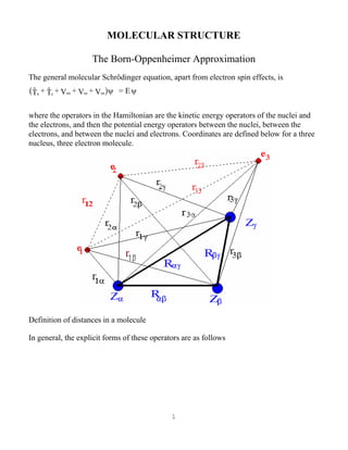
electrons, and between the nuclei and electrons. Coordinates are defined below for a three
nucleus, three electron molecule.
Definition of distances in a molecule
In general, the explicit forms of these operators are as follows

2. 2
n
2
2
e
i=1
2
e
i
2
nn
>
2
ee
i=1 j>i
2
ij
en
i
2
i
T =
2M
T =
2m
V =
Z Z e
R
V =
e
r
V =
Z e
r
nuclei
electrons
nuclei
electrons
nuclei electrons
α α
α
α β α
α β
αβ
α
α
α
∑
∑
∑ ∑
∑ ∑
∑ ∑ −
− ∇
− ∇
There is a repulsive interaction among the nuclear charges and a repulsive charge-charge
interaction among the electrons. However, the interaction potential between electrons and
nuclei is attractive, since the particles have opposite charges. This particular interaction
couples the motions of the electrons and the motions of the nuclei.
The wavefunctions that satisfy this Hamiltonian must be functions of both the
electron position coordinates and the nuclear position coordinates, and this differential
equation is not separable. In principle, true solutions could be found, but this is a
formidable differential equation to work with. An alternative is an approximate (but
generally a very good approximation) separation of the differential equation based upon
the very large difference between the mass of an electron and the masses of the nuclei.
The difference suggests that the nuclei will be sluggish in their motions relative to the
electron motions. Over a brief period of time, the electrons will "see" the nuclei as if fixed

3. 3
in space; the nuclear motions will be relatively slight. The nuclei, on the other hand, will
"see" the electrons as something of a blur, given their fast motions.
We may express the distinction between sluggish and fast particles in a
mathematical form by starting with an expansion of the wavefunction. To do this, let us
restrict attention to a diatomic molecule where there is only one coordinate, R, needed to
specify the separation of the nuclei. (There are, of course, six nuclear position
coordinates, but, after separating translation and rotation of the molecule, only one internal
coordinate remains.) A power series expansion about some specific point, Ro, is
ψ ψ
∂ψ
∂
∂ ψ
∂
( , , ) ( , , )
!
R r r R r r R R
R
R R
RR R R R
1 2 0 1 2 0
0
2 2
2
0 0
2
… … …= + − +
−
+
= =
b g b g
The electron position coordinates are designated r1, r2, etc. We will assume that the
first-derivative term in the expansion is the most important and that the higher order terms
may be neglected. By definition, the first derivative of the wavefunction is
∂ψ
∂
ψ δ ψ
δδR
=
R r r R r r
R R 0
o o
o= →
+ −
lim
, , , , , ,1 2 1 2… …b g b g
Our physical notion is that the electrons traverse a much greater distance for any
interval of time than do the nuclei because of the mass difference. Therefore, for some
small increment, δ, the electronic elements of the wavefunction will be much more
nearly the same at R = Ro
+δ and at R = Ro
than will the nuclear elements. This
means that the derivative above is largely determined by the change in the nuclear part of
the wavefunction, and that in turn suggests an approximate separation of the electronic and
nuclear motion parts of the problem.
To make the approximation that the electronic contributions to the derivative above
are zero requires first that the wavefunction be taken to be (approximately) a product of a
function of nuclear coordinates only, φ, and a function of electron coordinates, Ψ,at a
specific nuclear geometry. At the specific nuclear geometry, R = Ro, this is expressed as
ψ φ(R ,r ,r , ) (R ) (r ,r , )o 1 2 o
(R )
1 2
o
… …≅ Ψ
Notice the superscript Ro on the electronic wavefunction Ψ. It designates that this
function is for R = Ro, a specific point. A different R point would imply a different Ψ
function. From this, we must also have that

4. 4
ψ δ φ δ
φ δ φ
δδ
(R + ,r ,r , ) (R + ) (r ,r , )
R
= (r ,r , )
(R + ) (R )
= (r ,r , )
R
o 1 2 o
(R )
1 2
R=R
(R )
1 2
0
o o
(R )
1 2 R=R
o
o
o
o
o
… …
…
…
=
∂ψ
∂
−
∂φ
∂
→
Ψ
Ψ
Ψ
lim
Considering Ψ at all values of R is to view the electronic wavefunction as having a
dependence on the nuclear coordinate; the nuclear position coordinates are said to be
parameters and Ψ is said to have a parametric dependence.
If the product form of the wavefunction, ψ(R,r1,r2,...) = φ(R)Ψ (R)
(r1,r2,...), then we
can say something about the effect of the kinetic energy operators. Since Te acts only on
electron coordinates, then Teψ = φTeΨ (R)
. The nuclear kinetic energy term Tn affects both
functions since Ψ (R)
, the electronic wavefunction, retains a dependence on the nuclear
position coordinates as parameters. However, in Eq. (6), the derivative of the electronic
wavefunction with respect to the nuclear coordinates was approximated as zero. If the
second derivative is also approximated as zero, then
Tnψ (R,r1,r2,...) =Tn[φ(R) Ψ(R)
(r1,r2,...)] ≅ Ψ(R)
(r1,r2,...)Tnφ(R) (7)
Within this approximation, the Schrödinger equation is
φTeΨ(R)
+ Ψ(R)
TnN + φΨ(R)
(Vnn +Ven +Vee - E) = 0 (8)
Rearrangement of the terms in this expression leads to
φ[Te + Vee + Ven] Ψ(R)
+ Ψ(R)
(Tn + Vnn-E) φ = 0 (9)
Of the operators in brackets acting on Ψ (R)
, only one involves the nuclear position
coordinates. It is the term Ven giving the electron-nuclear attraction potential. In
Ψ(R)
, the nuclear coordinates are treated as parameters, and we can do the same for

5. 5
Ven, since it acts only on Ψ.
This allows us to write a purely electronic Schrödinger equation as
[Te + Vee + V(R)
en] Ψ(R)
(r1,r2,...) = E(R)
Ψ (R)
(r1,r2,...) (10)
The energy eigenvalue, E, must also have a parametric dependence on the nuclear
positions, as denoted by its superscript. That is, at each different R, there will be a
different Ven, and consequently a different Ψ and a different E.
Substitution of Eq. (10) into Eq. (9) yields
φE(R)
Ψ(R)
+ Ψ(R)
[Tn + Vnn - E]φ = 0 (11)
Since φ is a function only of nuclear position coordinates, then the following
separation results.
[Tn +(Vnn + E(R)
) -E] φ = 0 (12)
This is the Schrödinger equation for finding φ. The Hamiltonian consists of a kinetic
energy operator for the nuclear position coordinates, the repulsion potential between the
nuclei, and an effective potential, in the form of E(R)
, that gives the energy of the electronic
wavefunction as it depends on the nuclear position coordinates.
The Born-Oppenheimer approximation leads to a separation of the molecular
Schrödinger equation into a part for the electronic wavefunction and a part for the nuclear
motions, which is the Schrödinger equation for vibration and rotation. The essential
element of the approximation is Eq (7), namely that applying the nuclear kinetic energy
operator to the electronic wavefunction yields zero. The physical idea is that the light,
fast-moving electrons readjust to nuclear displacements instantaneously. This is the
reason the approximation produces an electronic Schrödinger equation for each possible
geometrical arrangement of the nuclei in the molecule (e.g., each value of R in the
diatomic we considered). We need only know the instantaneous positions of the nuclei,
not how they are moving, in order to find an electronic wavefunction, at least within this
approximation.
The approximation is put into practice by "clamping" the nuclei of a molecule of
interest. That means fixing their position coordinates to correspond to some chosen
arrangement or structure. Then, the electronic Schrödinger equation [Eq. (10)] is solved to

6. 6
give the electronic energy for this clamped structure. After that, perhaps, another structure
is selected, and the electronic energy is found by solving Eq. (10) once more. Eventually,
enough structures might be treated so that the dependence of the electronic energy on the
structural parameters is known fairly well. At such a point, the combination of E(R)
with
Vnn, which is a simple potential according to Eq (2), yields the effective potential for
molecular vibration. It is the potential energy for the nuclei in the field created by the
electrons.
The Born-Oppenheimer approximation is one of the best approximations in
chemical physics in the sense that it proves to be a valid approximation in most situations.
As with any approximation, of course, there is a limitation in its applicability, and in fact,
there are special phenomena that are associated with a breakdown in the Born-
Oppenheimer approximation. We may understand certain of the formal aspects of dealing
with a breakdown by comparing the form of a Born-Oppenheimer wavefunction with a
more general form. First, we note that any well-behaved function of two independent
variables can always be written as a sum of products of independent functions, as in
the following.
f(x, y) = c g (x)h (y)
i j
ij i j∑∑
The sums must be over sets of functions that are complete in the range of the
function f. In a power series expansion; for example, the gi and hi functions would be
polynomials in r and s, respectively. The cij's are the expansion coefficients. In effect, the
Born-Oppenheimer approximation uses such an expansion, but drops all but one term.
The wavefunction is just one product of a function of the nuclear coordinate(s) and a
function of the electron coordinate(s).
We realize that Eq (10) may have a number of different solutions, Just as the
harmonic oscillator has different energy states, the electrons in an atom or molecule may
have different states with different energies available. Also, the nuclear Schrödinger
equation, Eq (12), will have a number of different solutions. The set of these solutions is
complete in the range of the electronic-nuclear wavefunction, Ψ. So in principle, the non-
approximate wavefunction could be written as a sum of product functions,
Ψ = c
i j
ij i j∑∑ φ ψ
The Born-Oppenheimer approximation is to retain only one φΨ product, and so the
validity of the approximation depends on the coefficients of the other products (in the true

7. 7
Ψ) being significantly smaller. When this fails to be the case, the approximation breaks
down.
A possible means for dealing with a breakdown in the Born-Oppenheimer
approximation is to let the wavefunction include other products. For instance, if the
electronic energies of two Born-Oppenheimer electronic states became very close at some
point in the vibration of a molecule, then the nonapproximate wavefunction, or the non-
Born-Oppenheimer wavefunction, might properly be a superposition (or linear
combination) mostly of two products. As suggested by the curves below, the two product
functions would be the Born-Oppenheimer electronic-vibrational wavefunctions otherwise
obtained for the two different electronic states.
We might then say that the system has a nonvanishing probability of being in one or
the other "Born-Oppenheimer state," or that it could be hopping between. Of course, such
a description is entirely within the context of the Born-Oppenheimer approximation since
it presumes a separation of the electronic and nuclear motions. So important is the Born-
Oppenheimer approximation in chemistry that discussions are very often within the
context of the approximation (e.g., separation of electronic and nuclear motion), even if
not stated explicitly.