1. Nguyen 1
John Nguyen
1373244
The MLDA: Should I Go To A Bar On My 21st Birthday Or Stay Home Watching Netflix?
1. Abstract
In this paper, we answer to what degree the Minimum Legal Drinking Age (MLDA)
reduce the proportion of population that drinks and the population’s mortality rate. We address
these questions by utilizing both the National Health Interview Sample (NHIS) and National
Vital Statistics System (NVSS) dataset. By applying a regression discontinuity approach, we can
compare and contrast just to the left and right of the age 21 threshold. From this, we display how
both sides are demographically the same. Also, the MLDA does sharply reduce the number of
people around the age of 21 who drink, legally restricting them from buying alcohol, while doing
the same for mortality rates; the values we conclude are by 8% and upwards of 90 people per
100,000 respectively. From our IV estimates, we garner, depending on cause of death, 1 to 90
people per 100,000 change their alcohol habits which lead to their death.We conclude the MLDA
helps save lives by forcing people, withholding alcohol from teenagers until they reach 21
2. Introduction
This paper finds out to what extent the Minimum Legal Drinking Age (MLDA) reduces
the proportion of the population that drinks and the mortality. Answering these 2 questions has
significant value because we can determine whether the MLDA can be use as an instrumental

2. Nguyen 2
variable to learn if drinking alcohol is a cause of death. Over the last decade, there have been
groups like the Amethyst Initiative and Choose Responsibility who are pushing to reduce the
MLDA which would legalize alcohol consumption for people in the 18-20 age range, stating a
lower MLDA can reduce dangerous drinking.
We test whether the MLDA reduces the consumption of alcohol beverages and mortality
rates from National Health Interview Sample (NHIS) Adults and National Vital Statistics
System (NVSS) dataset.The NHIS provides us information on demographic dummy variables
from if they have a high school diploma to their race. It also provides data on observables on
alcohol consumption such as if they drink or not. The NVSS gives data on mortality rates per
100,000 by age and primary cause of death, ranging from homicide to motor vehicle accidents.
From these datasets, we are capable of composing age profiles of drinking and of death, mapping
out what age do we see increase and decreases in alcohol consumption and mortality.
We apply a fuzzy regression discontinuity method to these datasets to generate
regressions and scatterplots. By doing so, we can identify the causal difference between these
individuals, seen in the jump from the estimates, while establishing these individuals as
relatively the same except for in one chosen covariate. We continue with our RD design,
regressing our equation of whether they drink to find the 1st stage, using the polynomial order to
find the regression with the best fitted line. We also estimate our mortality equation to find the
Reduced Form, taking the two to compute the instrumental variable (IV) estimate. Finally, we
find our t-statistic to see if our IV estimate is statistically different from 0, requiring us to utilize
the Delta Method.

3. Nguyen 3
Our results show individuals on both sides of the threshold are similar in demographics
and crossing the threshold of 21 shows around an 8% increase in drinking and a jump in
mortality rates across the board, especially in death highly correlated with alcohol such as motor
vehicle accidents and suicide. Our IV estimates reinforce these results, displaying upwards of 90
people per 100,000 dying due to their change in drinking patterns. We see a small positive bias
associated with the the birthday effect of turning 21, overestimating how high cause of death
being correlated to being over 21 is, turning out to be insignificant in cause of death except for
alcohol poisoning. While some of these jumps are deem statistically insignificant, for instance
internal injuries or drug use, we see others like motor vehicle accidents (MVA) and alcohol
poisoning being statistically significant at the 99% confidence level. Most importantly, seeing
causes of deaths not highly correlated with alcohol like internal injuries remain relatively the
same while deaths highly correlated such as MVA jumps, we can infer our data and method of
estimating the MLDA effect to be effective.
3. Data
Our essential data comes from the National Health Interview Sample (NHIS) and
National Vital Statistics System (NVSS). Our NHIS dataset ranges from 1997 to 2007 with the
NHIS conducting surveys including questions on drinking participation, heavy episodic drinking,
and the number of days in the last month on which the person consumes alcohol. The NHIS
provides us information on demographic dummy variables such as if they have a high school
diploma, insurance, living wage, are married, employed, going to school, and if they are
hispanic, white, or black. It also supplies data on observables on alcohol consumption like days

4. Nguyen 4
to their 21st birthday and age, if they drink alcohol and how often in a month they drink. The
National Vital Statistics System is an inter-governmental system of sharing data on vital statistics
of the population of the United States . The NVSS death certificate records are a census of deaths
and include substantial detail on the cause of death. The NVSS gives data on mortality rates per
100,000 by age and primary cause of death, composing of internal and external conditions,
alcohol poisoning, homicide, suicide, motor vehicle accidents, drug use, and miscellaneous
external conditions. From these datasets, we compose age profiles of drinking and of death,
mapping out what age do we see increase and decreases in alcohol consumption and mortality.
These datasets are vital in understanding why the MLDA is 21 or why it exists. The
MLDA was developed under the National Minimum Drinking Age Act of 1984 as a way to cope
with the the rise in motor vehicle fatalities, correlated with the lowering of the MLDA in 29
states during 1970 through 1975. Opinions on whether the MLDA should be as low as 18 is
divisive, with the side against disputing young adults cannot control their consumption rate of
alcohol at such a young age with groups on the other side refuting this claim, believing it will
make the drinking problem amongst young adults and college students far worse.
One of these groups is the Amethyst Initiative, an organization made up of U.S. college
presidents and other higher education officials. A central argument of the Amethyst Initiative is
that the U.S. minimum legal drinking age policy results in more dangerous drinking than would
occur if the legal drinking age were lower. A companion organization called Choose
Responsibility explicitly proposes “a series of changes that will allow 18-20 year olds to
purchase, possess, and consume alcoholic beverages. Policies that change the ways in and extent

5. Nguyen 5
to which young people consume alcohol have the potential to affect the mortality rate of this
population substantially they dispute.
4. Methods
Estimating the effects of the minimum legal drinking age requires comparing the alcohol
consumption patterns and adverse event rates of young adults subject to the law with a similar
group of young adults not subject to it. A regression discontinuity (RD) design would be the
optimal method for estimating these effect, allowing us to find unbiased estimates base off the
data by assigning individuals to 2 groups, those under the 21 year old threshold within our
bandwidth and those above it.
The RD design functions under 2 assumptions, that there is a considerable jump in the
outcome of interest at the threshold point, age 21, and that both sides of the age threshold are
comparable and identical. In doing so, we establish our parameters for the scatter plot. We list
our bandwidth from the age of 19 through 23, believing it is best because our data points are
well-spaced while illustrating a definitive shape. Our bandwidth parameter is the most important
range to choose correctly, seeing as every year we deviate away from our center, the less precise
and impactful our results will become. Our binwidth is a 15 day period. While a 30 day period
would be more practical, we believe a 15 bin period avoids cluttering our data points together
and also form a resemblance of a pattern. Lastly, we create our y range. Our Y ranges from a 0.4
value to a 0.8, allowing us to focus on the main data points, and drawing our attention to the true
middle of our scatter plot. We believe these parameters give us the right blend of precision and
volume.

6. Nguyen 6
In a binary world, we would use a sharp regression discontinuity (SRD) design. Everyone
would comply to the MLDA, where if you are under 21 you have never had a drink while being
over 21 means you do drink alcohol. However, we have to assume that both people break the law
and drink before turning 21 or choose not to drink after turning 21. We make use of a fuzzy
regression discontinuity (RD) design, a RD design that differs from the SRD design since
treatment may or may not be receive even if the threshold is met.
We now move onto performing regressions on our equations, with whether you drink
being first. Our 1st Stage equation or drinks alcohol equation, first requires us to generate new
covariates.
DrinksAlcohol Over21i = ϕ0 + ϕ1 i + Days21ϕ2 i )+ (Over21ϕ3 i * Days21i + Birthdayϕ4 i
+ μi
The first variable we create is Over21, a dummy variable that represents if you pass the
threshold of age 21. It is the variable we have the most interest in because it measures the
increase in mortality when an individual turns 21 and is not limited by the MLDA. Next, we
establish the days_21 covariate, representing either how many days until you turn 21 or how far
past 21 you are. We generate the Over21*days_21 dummy variable, an interaction term which is
non-zero only when an individual turns 21. It serves to adjust for age-related changes in the
outcome variable while be flexible in filling out of scatter plot. We now implement a fitted line,
choosing between a linear, quadratic, or cubic specification. A dummy variable called Birthday
is use to capture the effect the day you turn 21 does to Over21. The linear specification is chosen
for simplicity’s sake; a more exact and flexible line can be found from the others due to more

7. Nguyen 7
covariates if desired. The 1st Stage Equation is expected to prove the assumption that the MLDA
reduces the level of alcohol consumption but we cannot guess to what degree.
We proceed to estimate the Reduced Form Equation or Mortality Rate Equation to learn
how far the MLDA reduces the mortality rate.
+ )+ +Over21 AgeMortalityi = π0 + π1 i + π2 ci
(Over21π3 i * Ageci
Birthdayπ4 i μi
Instead of Days_21, we generate a new covariate called . turns the age 21 intoAgeci
Ageci
a value of 0, giving us a way to properly calculate our mortality rate as its unit is per 100,000
people. We also generate a new interaction term, Over21* . As with Over21*days_21, thisAgeci
term only activates when a person turns 21. It also adjusts for age-related changes in the outcome
variable. A dummy variable called Birthday is again use to capture the effect the day you turn 21
does to Over21. We expect the Reduced Form equation to prove that while drinking alcoholic
beverages affects the outcome of death, the MLDA does reduce the mortality rate.
If we, economist, had the power choose our regression equation to see if our IV variable
affects the outcome variable of death, we would use:
+DrinksAlcoholMortalityi = π 0 + π 1 i μi
However, they are too many covariates to consider in the regression. We may run into an
Omitted Variable Bias (OVB) or Selection Bias by using such a simplistic equation. We come to
the conclusion an IV estimate is necessary to find the effects of drinking on the mortality rate.
Since we already have defined our 1st Stage and Reduced Form equation above, the only action
we need is to divide the reduced form estimate over the 1st Stage estimate.
βIV =
πi
ϕi

8. Nguyen 8
We compute the standard error by the Delta method, a method that combines both the 1st stage
and Reduced Form’s standard errors. Dividing the IV estimate by its standard error will give us a
t-statistic and whether it is less than or greater than a specific threshold point, we will know if
our IV estimate is statistically significant.
While the RD design is adept at finding significant differences between two seemingly
similar groups, there are two main conceptual concerns in the usage of a RD designs, sharp or
fuzzy. The first concern about RD designs is the possibility of other changes at the same
threshold point of the covariate. Such changes may affect the outcome, and these effects may be
misspecified to the treatment or another covariate. The second concern is manipulation of the
treatment status. If someone has knowledge of the threshold point, they may attempt to change
parts of their application to end up on the favorable side of the threshold. A common example for
the MLDA is a fake ID, allowing underage people the power to buy alcohol or order it in a bar.
5. Results
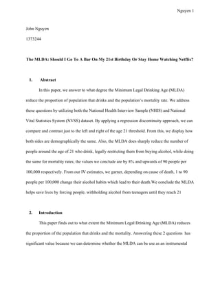
The first result we see is from Figure 1, detailing the Age Profile of Drinking. From our
fitted linear line, we see a steady increase in the percentage of people drinking alcohol from the
bandwidth range of 19 to 21. As we expect, a significant jump occurs at our threshold,
resembling an infinite slope. Interestingly enough, after the initial thrill the individual finds from
being able to legally buy and drink alcohol, the fitted line steadily increases as seen from the 19
through 21 range, though at a markedly slower pace. We can presume this occurs because the
allure of drinking or buying alcohol is greatly diminish since the individual can openly find and
buy it, a departure from convincing an older friend to buy or give you a glass. The age factor also

9. Nguyen 9
plays a role; the older you become, the more responsibility you’ll likely be due to having a
career, your body not being able to keep up with the drinking, etc.
From Table 1, our values from regression Equation 1 with different specifications and
whether a Birthday effect is there prove to be very significant. Whether you are or are not over
21, the estimated number of people who drink alcohol ranges from 54 to 56 percent, all at a 99%
confidence level. Being over 21 also increases the percentage of people who drink by as little as
9% and as high as 12%, all again being statistically significant at the 99% confidence level. The
higher you go in the polynomial order, the higher estimated percentage of people who drink on
their birthday is, demonstrating that the Over21 variable may be negatively bias by it.
Table 2 shows the results on whether people on the left side of the 21 year old threshold
are similar demographically to the people on the right, displaying they are similar in
non-alcoholic situations. Most non-alcoholic covariates for these groups do not deviate within
1%, the exception being married at a -2.5%. We also see it is the only non-alcoholic
demographic variable that has statistical significance, being at the 95% confidence level. We
conclude that people on both sides of the threshold are quite similar to each other besides who
gets to drink alcohol.
Figure 2 displays how effective and significant the MLDA is at reducing the general
mortality rate among young adults. Pre-21, the mortality rate shows some semblance of
progressing upward, though not quite consistently. However, right when you hit 21 and
experience the first 30 days after your 21st birthday, the mortality rate skyrockets, nearly
climbing at a 10% rate or 10 more deaths per 100,000 people compared to the previous data

10. Nguyen 10
point. A rapid decline in mortality begins right after these 30 days, seemingly stabilizing at a
gradual decreasing pacing within the 22nd birthday.
Figure 3 illustrates the decline in motor vehicle crashes for young adults before the RD
threshold. The older and more experience you are with a motor vehicle, the less likely you will
take dangerous risks while driving because of the additional wisdom and experience you accrue
while aging. However, another major spike occurs when the threshold point is cross, resulting in
a 20% or 4 more deaths per 100,000 people from the previous data point. An explanation that
more drunk or risky driving occurs because alcohol is now easily accessible to these individuals
is likely the cause. After the 21st birthday phenomena has subsides, individuals return to their
cautious ways pre-21, dropping down to 26 deaths per 100,000 people, 4 less than the pre-21’s
lowest point.
Figure 4 gives us a picture of how many lives are taken from alcohol poisoning per
100,000 people. With such a narrow y-range, being 0.5 to 3, we see a scatter plot with many
different trends. Climbs starting from the beginning of a birthday obviously occurs but other
climbs start in the middle of a year or near the end, suggesting these rises can be attribute to
popular holidays associated with drinking such as Fourth of July or Halloween. Unsurprisingly, a
spike occurs on the 21st birthday, solidifying that MLDA is reducing the mortality rate among
young adults.
Table 3 and 4 detail estimates of increases in death both overall and in each subcategory
of death, with and without a birthday effect. First, we recognize, in Table 4, if all covariates are
zero, the estimated number of deaths that occur whether you are 21 or not is about 94 per
100,000, found to be significant at a 99% confidence level. As we go down the table, the most

11. Nguyen 11
common ways of death, such as external injuries and motor vehicle accidents are high in death
counts, with them respectively at 74 and 30 deaths per 100,000 at a 99% confidence level. Even
unusual deaths such as drugs or alcohol poisoning, clocking in at 4 and 1 death per 100,000
people, are statistically significant at the 99% confidence level. We see that the causes of death
which have statistical significance from being over 21 are in external injuries, alcohol poisoning,
suicide, and motor vehicle accidents. Each are heavily associated with drinking, with a
handicapped mind not being able to make sound judgment calls on avoiding physical injuries or
fighting against the negative thoughts that fill one’s head when contemplating suicide. Motor
vehicle accidents and alcohol poisoning were already proven to be statistically significant in the
figures above, seeing as a drunk driver is more likely to get into a vehicle accident and alcohol
being require to have alcohol poisoning. These 4 causes of death add an additional 7, 0.3, 2, and
4 deaths per 100,000 people. Now for the birthday effect, it only has statistical significance for
alcohol poisoning, adding an extra 1 death per 100,000 at a 99% confidence level. Table 3
matches up with Table 4’s values for the most part except when it comes down to the Over21
covariate. Without the birthday effect to sponge the 21st birthday, death per 100,000 increases
across the board for all causes.
Asides from the RD designs and regressions, we found the effect of the MLDA on
mortality in terms of per person drinking using an IV estimate approach. As seen in Table 5, our
IV estimates are showing the number of people who alter their drinking patterns after passing the
MLDA threshold point, with whopping 85 to 90 people per 100,000 dying from external injuries
or in general because they are allow to drink freely. While the other IV estimates are not nearly
as dramatic as the other 2 causes of death, there is an indication the MLDA is the main limitator

12. Nguyen 12
as to why people chose not to drink. The most likely case is they rarely drank before turning 21
and only do so because they have legal access to it anywhere. Also seen in the table are
t-statistical scores, we find external, alcohol poisoning, suicide, and motor vehicle accidents, and
death in general being statistically different from zero.
6. Conclusion
Our paper set out to discover how effective the Minimum Legal Drinking Age (MLDA)
cuts down the population of people who drinks alcohol and the mortality rate. Seeing as the
MLDA did both effectively, we can start thinking of the MLDA as a strong instrumental variable
(IV) to figure out if drinking causes death. We are able to prove the MLDA reduces the
proportion of people drinking and the mortality rate by inputting the National Health Interview
Sample (NHIS) and the National Vital Statistics System (NVSS) dataset into our regressions.
These datasets provide crucial demographic and mortality observables respectively, giving us the
ability to compose age profiles of the population. Utilizing a fuzzy regression discontinuity
(FRD) method, we are able to both find the threshold difference between our two assignment
groups while making the groups comparable. We regress equations to find a linear fitted line, the
1st Stage and Reduced Form effect, and the IV estimate. From our results, we see passing the
threshold point of age 21 displays an 8% increase in drinking and mortality rates for all causes of
deaths to increase, with death cause by alcoholic and turning 21 being highly correlated.
Additionally, a number of our IV estimates are statistically different from zero. With deaths not
correlated with alcohol seeing a much less significant jump and being statistically insignificant,

13. Nguyen 13
we conclude our methods and datasets are correctly chosen and effective in demonstrating the
positive effects of the MLDA on whether a person drinks and the mortality rate.
However, using and accepting an IV estimator requires 2 assumptions to have validity.
First, the estimate must have a non-zero first stage; there must be voluntary compliance into
whether or not you drink. The second assumption is the instrumental variable (turning 21) must
directly affect your outcome variable (death) only through the instrumented variable (drinking).
While this is mainly the case, many fringe situations occur which can break this assumption and
potentially invalidate the IV estimate. Say someone turns 21 but does not enjoy drinking. They
still enjoy the company of friends and acquaintances who do drink so they have no reason to not
hang out with them at a bar. If, when driving home from the bar, they are in a car accident, this
would invalidate our assumption. Once this view is spoken and receives sensible agreements
amongst other economic peers, the IV estimate is now thrown out the window because going to
and from a bar when other people are drinking raises the chances of being in a motor vehicle
accident, thus circumventing the instrumental to instrumented to outcome variable path required
of an IV estimate. However, as economists, we must learn to be practical and compromising,
recognizing the niche situations and whether an IV estimate can be generally acceptable.