Geophys. J. Int.-2016-Bodin-605-29

Geophysical Journal International
Geophys. J. Int. (2016) 206, 605–629 doi: 10.1093/gji/ggw124
Advance Access publication 2016 April 4
GJI Seismology
Imaging anisotropic layering with Bayesian inversion
of multiple data types
T. Bodin,1,2
J. Leiva,1
B. Romanowicz,1,3,4
V. Maupin5
and H. Yuan6
1Berkeley Seismological Laboratory, 215 McCone Hall, UC Berkeley, Berkeley CA 94720-4760, USA. E-mail: thomas.bodin@ens-lyon.fr
2Univ Lyon, Universite Lyon 1, Ens de Lyon, CNRS, UMR 5276 LGL-TPE, F-69622 Villeurbanne, France
3Insitut de Physique du Globe de Paris (IPGP), 1 Rue Jussieu F-75005 Paris, France
4College de France, 11 place Marcelin Berthelot, F-75231 Paris, France
5Department of Geosciences, University of Oslo, P.O. Box 1047, Blindern, Oslo 0316, Norway
6Department of Earth and Planetary Sciences, Macquarie University, New South Wales 2109, Australia
Accepted 2016 March 31. Received 2016 March 31; in original form 2015 September 1
S U M M A R Y
Azimuthal anisotropy is a powerful tool to reveal information about both the present structure
and past evolution of the mantle. Anisotropic images of the upper mantle are usually obtained
by analysing various types of seismic observables, such as surface wave dispersion curves
or waveforms, SKS splitting data, or receiver functions. These different data types sample
different volumes of the earth, they are sensitive to different length scales, and hence are
associated with different levels of uncertainties. They are traditionally interpreted separately,
and often result in incompatible models. We present a Bayesian inversion approach to jointly
invert these different data types. Seismograms for SKS and P phases are directly inverted using
a cross-convolution approach, thus avoiding intermediate processing steps, such as numerical
deconvolution or computation of splitting parameters. Probabilistic 1-D profiles are obtained
with a transdimensional Markov chain Monte Carlo scheme, in which the number of layers, as
well as the presence or absence of anisotropy in each layer, are treated as unknown parameters.
In this way, seismic anisotropy is only introduced if required by the data. The algorithm is
used to resolve both isotropic and anisotropic layering down to a depth of 350 km beneath
two seismic stations in North America in two different tectonic settings: the stable Canadian
shield (station FFC) and the tectonically active southern Basin and Range Province (station
TA-214A). In both cases, the lithosphere–asthenosphere boundary is clearly visible, and
marked by a change in direction of the fast axis of anisotropy. Our study confirms that
azimuthal anisotropy is a powerful tool for detecting layering in the upper mantle.
Key words: Inverse theory; Body waves; Surface waves and free oscillations; Seismic
anisotropy; North America.
1 I N T RO D U C T I O N
Seismic anisotropy in the crust and upper mantle can be produced
by multiple physical processes at different spatial scales. In the
mantle, plastic deformation of olivine aggregates results in a crys-
tallographic preferential orientation (CPO) of minerals, and pro-
duces large-scale seismic anisotropy that can be observed seismo-
logically. These observations are usually related to the strain field,
and interpreted in terms of either present day flow, or ‘frozen’ flow
from the geological past. Furthermore, the spatial distribution of
cracks, fluid inclusions, or seismic discontinuities can induce appar-
ent anisotropy, called shape-preferred orientation (SPO) anisotropy
(Crampin & Booth 1985; Backus 1962). In this way, anisotropic
properties of rocks are closely related to their geological history
and present configuration, and hence reveal essential information
about the Earth’s structure and dynamics (e.g. Montagner & Guillot
2002).
Observations of seismic anisotropy depend on the 21 parameters
of the full elastic tensor. However, all these parameters cannot be
resolved independently at every location, and seismologists usually
rely on simplified assumptions on the type of anisotropy, namely
hexagonal symmetry. This type of anisotropy is defined by the five
Love parameters of transverse isotropy (A, C, F, L, N) and two angles
describing the direction of the axis of symmetry (Love 1927). Most
seismological studies assume one of two types of anisotropy: (1)
radial anisotropy, where the axis of hexagonal symmetry is vertical
and with no azimuthal dependence and (2) azimuthal anisotropy,
where the axis of hexagonal symmetry is horizontal with unknown
direction. Retrieving the tilt of the hexagonal axis of symmetry is in
principle possible (Montagner & Nataf 1988; Plomerová & Babuˇska
C The Authors 2016. Published by Oxford University Press on behalf of The Royal Astronomical Society. 605
byguestonSeptember6,2016http://gji.oxfordjournals.org/Downloadedfrom

606 T. Bodin et al.
2010; Xie et al. 2015), but in practice difficult, due to limitations in
the available azimuthal coverage, trade-offs with other competing
factors, such as tilted layers in the case of body waves and non-
uniqueness of the solution in the case of surface waves inversion.
Azimuthal anisotropy in the crust and upper mantle can be ob-
served from different seismic measurements, sampling the Earth
at different scales: surface wave observations, core-refracted shear
wave (SKS) splitting measurements and receiver functions. The lat-
ter two methods rely on relatively high-frequency teleseismic body
waves measurements, and therefore can provide good lateral resolu-
tion in those areas of continents where broad-band station coverage
is dense, if good azimuthal coverage is available.
Receiver functions have the potential of resolving layered
anisotropic structure locally. Large data sets from single seismic
stations have been used to image both anisotropic and dipping struc-
tures primarily at crustal depths (e.g. Kosarev et al. 1984; Levin &
Park 1997; Peng & Humphreys 1997; Savage 1998; Farra & Vinnik
2000; Frederiksen & Bostock 2000; Leidig & Zandt 2003; Vergne
et al. 2003; Schulte-Pelkum & Mahan 2014; Audet 2015; Bianchi
et al. 2015; Liu et al. 2015; Vinnik et al. 2016). Harmonic decompo-
sition methods have been developed to distinguish the contributions
from isotropic and anisotropic discontinuities, and dipping layers
(Kosarev et al. 1984; Girardin & Farra 1998; Bianchi et al. 2010).
Shear wave splitting measurements in core-refracted phases (SKS
and SKKS) provide constraints on the integrated effect of azimuthal
anisotropy across the thickness of the mantle beneath a single sta-
tion (e.g. Vinnik et al. 1984, 1989; Silver & Chan 1991; Vinnik
et al. 1992; Silver 1996; Long & Silver 2009), but depth resolu-
tion is generally poor, even when considering finite-frequency ker-
nels (Chevrot 2006), and there are trade-offs between the strength
of anisotropy and the thickness of the anisotropic domain. Due
to the lack of sufficient azimuthal coverage to distinguish more
than one layer, shear wave splitting measurements are usually in-
terpreted under the assumption of a single layer of anisotropy with
a horizontal axis of symmetry. We note however several attempts
to map multiple layers as well as a dipping fast axis (Silver &
Savage 1994; Levin et al. 1999; Hartog & Schwartz 2000; Yuan
et al. 2008).
Surface wave tomographic inversions provide constraints on
both radial (Gung et al. 2003; Plomerová et al. 2002; Nettles &
Dziewoński 2008; Fichtner et al. 2010) and azimuthal anisotropy at
the regional (Forsyth 1975; Simons et al. 2002; Deschamps et al.
2008; Beghein et al. 2010; Fry et al. 2010; Adam & Lebedev 2012;
Darbyshire et al. 2013; Zhu & Tromp 2013; Legendre et al. 2014;
Köhler et al. 2015) and global scale (Tanimoto & Anderson 1985;
Montagner & Nataf 1986; Trampert & van Heijst 2002; Trampert
& Woodhouse 2003; Debayle et al. 2005; Beucler & Montagner
2006; Visser et al. 2008; Debayle & Ricard 2012, 2013; Yuan &
Beghein 2013, 2014). Surface waves provide better vertical resolu-
tion than SKS data, but are limited in horizontal resolution due to
the long wavelengths. Still, the depth range where vertical resolu-
tion is achieved depends on the frequency range considered (longer
periods sample deeper depths), as well as the type of surface waves
considered. Most studies are based on the analysis of fundamental
mode surface wave dispersion up to about 200–250 s, which have
good resolution down to lithospheric depths, although inclusion of
surface wave overtones can improve resolution at depth (e.g. Yuan
& Beghein 2014; Durand et al. 2015).
These three different data types are therefore characterized by
different sensitivities to structure. They are modelled with different
approximations of the wave equation, and associated with different
noise levels. A well-known problem is that they often provide incom-
patible anisotropic models, and lead to contradictory interpretations.
For example, surface waves and SKS waves sample different vol-
umes in the earth, and SKS splitting measurements often disagree
with predictions made from surface wave tomographic models (e.g.
Montagner et al. 2000; Conrad et al. 2007; Becker et al. 2012; Wang
& Tape 2014). This discrepancy can be explained by the progressive
loss of resolution of fundamental mode surface waves below depths
of 200–250 km. Furthermore, body waves and surface waves are
measured in different frequency bands, and hence are sensitive to
structure at different wavelengths. The sharp discontinuities that can
be resolved by receiver functions are usually mapped into apparent
radial anisotropy in smooth models constructed from surface waves
(Capdeville et al. 2013; Bodin et al. 2015).
In order to improve resolution in anisotropy, several studies have
proposed joint inversion algorithms combining body waves and sur-
face waves. Marone & Romanowicz (2007), Yuan & Romanowicz
(2010b) and Yuan et al. (2011) iteratively combined 3-D waveform
tomography (including fundamental surface waves and overtones)
with constraints from shear wave splitting data in North Amer-
ica. They showed that by incorporating body waves, the anisotropy
strength significantly increases at the asthenospheric depth, while
the directions remain largely unchanged. However, these models
are obtained by linearized and damped inversions, where the pro-
duced seismic models strongly depend on choices made at the out-
set (reference model, regularization). This precludes propagation
of uncertainties from observations to inverted models, and hence
makes the interpretation difficult. In another approach, Vinnik et al.
(2007), Obrebski et al. (2010) and Vinnik et al. (2014) performed
a 1-D Monte Carlo joint inversion of SKS and receiver functions
at individual broad-band stations, but long-wavelength information
from surface waves was not used in this case. Therefore, two main
challenges remain in anisotropic imaging:
(i) To our knowledge, azimuthal variations of surface wave dis-
persion measurements have never been inverted jointly with receiver
functions.
(ii) It is difficult to jointly invert different data types, as inverted
models strongly depend on the choice of parameters used to weigh
the relative contribution of each data sets in the inversion.
In this work, we address these issues with a method for 1-D in-
version under a seismic station. We jointly invert Rayleigh wave
dispersion curves with their azimuthal variations, together with
converted body waves and SKS data. For body waves, standard
inversion procedures are usually based on secondary observables,
such as deconvolved waveforms (receiver functions) or splitting
parameters for SKS data. Here, we directly invert the different com-
ponents of seismograms with a cross-convolution approach, as this
allows us to better propagate uncertainties from recorded wave-
forms towards a velocity model (Menke & Levin 2003; Bodin et al.
2014). We cast the problem in a Bayesian framework, and explore
the space of earth models with a Markov chain Monte Carlo algo-
rithm. This allows us to deal with the non-linear and non-unique
nature of the problem, and quantify uncertainties. The solution is
a probabilistic 1-D profile describing shear wave velocity, strength
of azimuthal anisotropy and fast axis direction, at each depth. We
use a transdimensional formulation where the number of layers as
well as the presence of anisotropy in each layer are treated as free
variables.

Bayesian imaging of anisotropic layering 607
2 M E T H O D O L O G Y
2.1 Model parametrization
The full elastic tensor of 21 parameters is usually described with
the so-called Voigt notation 6 × 6 symmetric matrix Cmn (Maupin
& Park 2007). An elastic medium with hexagonal (i.e. cylindrical)
symmetry and horizontal axis of symmetry is called a horizontal
transverse isotropic model (HTI), and is usually defined by the five
Love parameters of transverse isotropy A, C, F, L, N (Love 1927):
Cmn =
⎛
⎜
⎜
⎜
⎜
⎜
⎜
⎜
⎜
⎜
⎜
⎝
A F (A − 2N) 0 0 0
F C F 0 0 0
(A − 2N) F A 0 0 0
0 0 0 L 0 0
0 0 0 0 N 0
0 0 0 0 0 L
⎞
⎟
⎟
⎟
⎟
⎟
⎟
⎟
⎟
⎟
⎟
⎠
(1)
Here, axis 3 is vertical and axis 2 is the horizontal axis of symmetry.
A, C, N and L can be related to P- and S-wave velocities in different
directions. If ψfast is the angle of the fast axis relative to North, the
velocity of Swaves propagating horizontally and polarized vertically
(SV waves) is given by (Crampin 1984):
ρV 2
sv(ψ) =
(L + N)
2
+
(L − N)
2
cos(2(ψ − ψfast)) (2)
where ψ is the direction of propagation relative to North. The
velocity of P waves and SH waves propagating in the horizontal
plane are a bit more complicated as they contain cos(4ψ) terms.
The corresponding expressions can be found in Crampin (1984).
In this work, instead of using elastic parameters, we follow the
notation used in most body waves studies, and parametrize our
model in terms of seismic velocities, where the isotropic component
is given by the values of Vs and Vp, and the anisotropic component is
defined in terms of ‘peak to peak’ level of anisotropy δVp, δVs (e.g.
Farra et al. 1991; Romanowicz & Yuan 2012). These parameters are
related to the five elastic parameters A, C, F, L, N by the following
expressions:
C
ρ
= Vp +
δVp
2
2
,
A
ρ
= Vp −
δVp
2
2
, (3)
L
ρ
= Vs +
δVs
2
2
,
N
ρ
= Vs −
δVs
2
2
, (4)
The elastic parameter F controls the velocity along the direction
intermediate between the fast and the slow directions. It is com-
mon to parametrize it with the fifth parameter η = F/(A − 2L),
which we set to one (i.e. F = A − 2L) as in PREM (Dziewonski &
Anderson 1981). Following Obrebski et al. (2010), we also impose
Vp/VS = 1.7 for the sake of simplicity. The density ρ is calculated
through the empirical relation ρ = 2.35 + 0.036(Vp − 3)2
as done in
Tkalˇcić et al. (2006). In order to reduce the number of parameters,
the ratio between the percentage of anisotropy for the compres-
sional and shear waves (δVp/Vp)/(δVs/Vs) is fixed at 1.5 based on
the analysis of published data for the upper mantle (Obrebski et al.
2010). Here, we acknowledge that surface waves and normal modes
are sensitive to parameter η, Vp and density (Beghein & Trampert
2004; Beghein et al. 2006; Kustowski et al. 2008), and that we could
have easily treated these parameters as unknowns in the inversion.
It has been demonstrated that η trade-offs with P-wave anisotropy
(Beghein et al. 2006; Kustowski et al. 2008), implying that making
assumptions on either one of these parameters will likely affect re-
sults and inferred model uncertainties. Although one could invert
for the entire elastic tensor in each layer, this would be at increased
computational cost. Here instead, we use these empirical scaling
relations to determine the least constrained parameters.
As shown in Fig. 1, our model is parametrized in terms of a stack
of layers with constant seismic velocity. In our transdimensional
formalism, the number of unknowns is variable, as we want to
explain our data sets with the least number of free parameters. Each
layer can be either isotropic and described solely by its shear wave
velocity Vs (in this case, δVs = 0), or azimuthally anisotropic and
described by three parameters: Vs, δVs and ψfast the direction of
the horizontal fast axis relative to the north. The layer thickness is
also variable and the last layer is a half-space. The other parameters
(ρ, Vp, δVs) are given by the scaling relations mentioned above.
The number of layers k as well as the number of anisotropic layers
l ≤ k are free parameters in the inversion (see Fig. 1). Therefore,
the complete model to be inverted for is defined as
m = [z, Vs, δVs, fast], (5)
where the vector z = [z1, . . . , zk] represents the depths of the k dis-
continuities, Vs is a vector of size k and δVs, fast are vectors of size
l. The total number of parameters in the problem (i.e. the dimension
of vector m) is therefore 2(k + l). We shall show how a Monte Carlo
algorithm can explore different types of model parametrizations.
As in any data inference problem, it is clear that observations can
always be better explained with more model parameters (with l and
k large). However, we will see that in a Bayesian framework, overly
complex models with a large number of parameters have a lower
probability and are naturally penalized. Between a simple and a
complex model that fit the data equally well, the simple one will be
preferred. With this formulation, anisotropy will only be included
into the model if required by the data.
When inverting long-period seismic waves, this flexible approach
to parametrizing an elastic medium allowed us to quantify the trade-
off between vertical heterogeneities (lots of small isotropic layers)
and radial anisotropy (fewer anisotropic layers) (Bodin et al. 2015).
This trade-off can be broken by adding higher frequency observa-
tions from body waves, thus allowing a consistent interpretation of
different data types.
2.2 The data
For surface waves, we assume that some previous analysis (local or
tomographic) provides us with the phase velocity dispersion at the
station and its azimuthal variation. To first order, the phase velocity
of surface waves in an anisotropic medium can be written as:
C(T, ψ) = C0(T ) + C1(T ) cos(2ψ) + C2(T ) sin(2ψ)
+ C3(T ) cos(4ψ) + C4(T ) sin(4ψ) (6)
where T is the period and ψ is the direction of propagation relative to
the north (Smith & Dahlen 1973). For fundamental mode Rayleigh
waves, the 2ψ terms C1 and C2 are sensitive to depth variations
of Vs, δVs and ψfast, and the 4ψ terms are negligible, due to the
low amplitude of sensitivity kernels (Montagner & Tanimoto 1991;
Maupin & Park 2007). We will therefore only invert C0(T), C1(T)
and C2(T), and ignore 4ψ terms.
For body waves, recorded seismograms of P and SKS phases
for events coming from different backazimuths will be inverted.
To reduce the level of noise in P waveforms, individual events
coming from the same regions (i.e. within a small backazimuth–

608 T. Bodin et al.
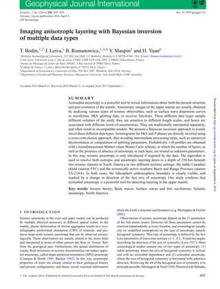
Figure 1. The 1-D model is parametrized with a variable number of layers, which can be either isotropic and described by one parameter Vs (light grey), or
anisotropic and described by three parameters Vs, δVs and ψfast (dark grey). As our Monte Carlo parameter search algorithm samples the space of possible
models, different types of jumps (black arrows) are used to explore different geometries (change the depth of a discontinuity, add/remove an isotropic layer
and add/remove anisotropy to an existing layer).
distance range) will be stacked (Kumar et al. 2010). This reduces
the number of waveforms that need to be modelled by the inversion
algorithm, and hence reduces computational cost. The range of ray
parameters and backazimuths in each bin directly impacts the type
of errors in the stacked seismograms. A large bin allows one to
include more events resulting in ambient and instrumental noise
reduction, although 3-D and moveout effects also become more
significant in this case. A compromise needs to be found for each
experiment when defining the range of incident rays.
When analysing azimuthal variations of receiver functions or
SKS waveforms, a number of studies decompose waveforms into
angular harmonics, in order to isolate π-periodic variations that
can be explained by azimuthal anisotropy (e.g. Kosarev et al. 1984;
Girardin & Farra 1998; Farra & Vinnik 2000; Bianchi et al. 2010;
Audet 2015). However in this work, waveforms will not be filtered to
isolate π-periodic azimuthal variations, and our ‘raw’ data will also
contain azimuthal variations due to 3-D effects, such as dipping dis-
continuities (associated with 2π-periodic variations). These varia-
tions will be accounted for as data noise in our Bayesian formulation.
2.3 The forward calculation
We use a forward modelling approach, where at each step of a Monte
Carlo sampler, a new model m, as defined in Fig. 1, is tested, and
synthetic data predicted from this model are compared to actual
measurements.
For Rayleigh waves, dispersion curves and their azimuthal vari-
ations are computed with a normal mode formalism in a spherical
Earth (Smith & Dahlen 1973). The term C0(T) is computed in
a fully non-linear fashion with a Runge–Kutta matrix integration
(Saito 1967; Takeuchi & Saito 1972; Saito 1988). However, the re-
lation linking the model parameters to the terms C1(T) and C2(T) is
linearized around the current model m averaged azimuthally, which
is radially anisotropic (Maupin 1985; Montagner & Nataf 1986).
A detailed description of the procedure is given in Appendix A.
We acknowledge that we are limited to a linear approximation of
the problem for azimuthal terms. Future work includes treating the
problem fully non-linearly, and computing dispersion curves exactly
as done in Thomson (1997).
For body waves, that is, P and SKS waveforms, the impulse re-
sponse of the model m to an incoming planar wave with frequency
ω and slowness p is computed with a reflectivity propagator-matrix
method (Levin & Park 1998). The transmission response is calcu-
lated in the Fourier domain at a number of different frequencies.
Particle motion at the surface is then obtained by an inverse Fourier
transform. The algorithm is outlined in detail in Park (1996) and
Levin & Park (1997). The computational cost of this algorithm
varies linearly with the number of frequencies ω and the number of
layers in m.
We note here that the Rayleigh wave dispersion curves are com-
puted in a spherical earth whereas body waves are predicted for a
flat Earth, which may produce some inconsistencies. However, P
and SKS waves propagate almost vertically under the station, and
hence are only poorly sensitive to the earth sphericity.
2.4 Bayesian inference
We cast our inverse problem in a Bayesian framework, where infor-
mation on model parameters is represented in probabilistic terms
(Box & Tiao 1973; Smith 1991; Gelman et al. 1995). Geophysi-
cal applications of Bayesian inference are described in Tarantola
& Valette (1982), Duijndam (1988a,b) and Mosegaard & Tarantola
(1995). The solution is given by the a posteriori probability distri-
bution (or posterior distribution) p(m|dobs), which is the probability
density of the model parameters m, given the observed data dobs.
The posterior is given by Bayes’ theorem:
posterior ∝ likelihood × prior (7)
p(m | dobs) ∝ p(dobs | m)p(m). (8)
The term p(dobs|m) is the likelihood function, which is the prob-
ability of observing the measured data given a particular model.
p(m) is the a priori probability density of m, that is, what we know
about the model m before measuring the data dobs.
In a transdimensional formulation, the number of unknowns (i.e.
the dimension of m) is not fixed in advance, and so the posterior
is defined across spaces with different dimensions. Below we show
how the likelihood and prior distributions are defined in our prob-
lem, and how a transdimensional Monte Carlo sampling scheme
can be used to generate samples from the posterior distribution,
that is, an ensemble of vectors m whose density reflects that of the
posterior distribution.
2.5 The likelihood function
The likelihood function p(dobs|m) quantifies how well a given model
m can reproduce the observed data. Assuming that different data
types are measured independently, we can write:
p(dobs | m) = p(C0 | m)p(C1 | m)p(C2 | m)p(dp | m)p(dSKS | m)
(9)

where C0, C1 and C2 are surface wave dispersion curves (see eq. 6),
and where dP and dSKS are seismograms observed for P and SKS
waves.
2.5.1 Surface wave measurements
For Rayleigh wave dispersion curves (C0(T), C1(T) and C2(T)),
we assume that data errors (both observational and theoretical)
are not correlated and are distributed according to a multivariate
normal distribution with zero mean and variances σC0
, σC1
and
σC2
respectively. For C0(T), the likelihood probability distribution
writes:
p(C0 | m) =
1
(
√
2πσC0
)n
× exp
− C0 − c0(m) 2
2σ2
C0
, (10)
where n is the number of data points, that is, the number of periods
considered and c0(m) is the dispersion curve predicted for model
m. In the same way, we define the likelihoods for 2ψ terms p(C1|m)
and p(C2|m).
2.5.2 A cross-convolution likelihood function for body waves
In traditional receiver function analysis, the vertical component
of a P waveform is deconvolved from the horizontal components,
to remove source and distant path effects (Langston 1979). The
resulting receiver function waveform can then be inverted for a 1-D
seismic model, by minimizing the difference between observed and
predicted receiver functions:
φ(m) =
Hobs(t)
Vobs(t)
−
h(t, m)
v(t, m)
, (11)
where Vobs(t) and Hobs(t) are observed seismograms for vertical
and radial components, and v(t, m) and h(t, m) are the vertical
and radial impulse response functions of the near receiver structure,
calculated for model m. Here, the division sign represents a spectral
division, or deconvolution. Although receiver function analysis has
been extensively used for years, there are two well-known issues:
(i) The deconvolution is a numerical unstable procedure that
needs to be stabilized (e.g. water level deconvolution; use of a
low-pass filter). This results in a loss of resolution, which trade-offs
with errors in the receiver function.
(ii) Uncertainties in receiver functions are therefore difficult to
estimate.
These two issues have been well studied in the last decades (e.g.
Park & Levin 2000; Kolb & Lekić 2014). Following Menke & Levin
(2003), we propose a misfit function for inverting converted body
waves without deconvolution, by defining a vector of residuals as
follows (Bodin et al. 2014):
r(m, t) = v(t, m) ∗ Hobs(t) − h(t, m) ∗ Vobs(t), (12)
where the sign ∗ represents a time-domain discrete convolution.
The vector r is a function of observed and predicted data defined
such that the unknown source function and distant path effects
are accounted for in both terms giving r = 0 for the true model
parameters m and zero errors. The norm r(m) is used as a misfit
function, and is equivalent to the distance between observed and
predicted receiver functions in (11). However, (1) it does not involve
any deconvolution and no damping parameters need to be chosen;
(2) the probability density function for r(m, t) can be estimated from
errors statistics in observed seismograms. If we assume that errors
Table 1. Possible component pairs that can be used in an inversion based
on the cross-convolution misfit function defined by Menke & Levin (2003).
These four different pairs have complementary sensitivities to seismic dis-
continuities and anisotropy. The advantage of a cross-convolution misfit
function is that these different data types can all be inverted in the same
manner.
Conversions PSV R-Z components Phase P
Conversions PSH T-Z components Phase P
Conversions SP R-Z components Phase S
SKS splitting R-T components Phases SKS and SKKS
in Vobs(t) and Hobs(t) are normally distributed and not correlated
(Gaussian white noise), we have (see Appendix B for details):
p(r | m) =
1
(
√
2πσp)n
× exp
− r(m) 2
2σ2
p
. (13)
For a given P waveform dp = [Vobs(t), Hobs(t)], resulting from a
stack of events coming from similar distances and backazimuths,
we use the distribution in (13) as the likelihood function p(dp|m) to
quantify the level of agreement between observations and the pre-
dictions from a proposed earth model. Then, we combine a number
of stacked waveforms measured at different backazimuths–distance
bins by simply using the product of their likelihoods, thus resulting
in a joint inversion of several waveforms with different incidence
angles. A clear advantage is that we can use the same formalism
to construct the likelihood function for SKS waveforms p(dSKS|m),
as the vertical and radial components need simply be replaced by
radial and transverse. The cross-convolution misfit function can
also be used for incoming S waves, that is, SP receiver functions,
or transverse receiver functions, where the vertical component of a
P waveform is deconvolved from its transverse component (see
Table 1). In this way, we can integrate various data types in a
consistent manner, with different sensitivities to the isotropic and
anisotropic seismic structure beneath a station.
However, we acknowledge here that p(r|m) is not exactly a like-
lihood function per se, as it does not represent the probability dis-
tribution of data vectors Vobs(t) and Hobs(t), but rather the distri-
bution of a vector of residuals conveniently defined. In a Bayesian
framework, the vector of residuals is usually defined as a difference
between observed data and predicted data: r(m) = dobs − dest(m).
In this case, the distribution of r for a given model m gives the
distribution of the observed data (p(r|m) = p(dobs|m)). However
here, p(r|m) does not strictly represent the probability of observing
the data, and hence cannot be strictly interpreted as a likelihood
function. We note that this way of approximating the likelihood by
the distribution of some residuals is also used by Stähler & Sigloch
(2014), who proposed a Bayesian moment tensor inversion based
on a cross-correlation misfit function. For a fully rigorous Bayesian
approach to inversion of converted body waves, we refer the reader
to Dettmer et al. (2015), who treated the source time function as an
unknown in the problem.
2.6 Hierachical Bayes
The level of data errors for different data sets (σC0
, σC1
, σC2
, σp,
σSKS, etc.) determines the width of the different Gaussian likelihood
functions in (9), and hence the relative weight given to different
data types in the inversion. Here, the level of noise also accounts
for theoretical errors, that is, the part of the signal that we are not
able to explain with our simplified 1-D parametrization and forward
theory (Gouveia & Scales 1998; Duputel et al. 2014). For example,
surface waves are sensitive to a larger volume around the station,

610 T. Bodin et al.
compared to higher frequency body waves arriving at the station
with a near vertical incidence angle. Lateral inhomogeneities in the
earth will then produce an incompatibility between these two types
of observations, which here will be treated as data uncertainty.
In this work, we use a Hierarchical Bayes approach, and treat
noise parameters as unknown in the inversion (Malinverno & Briggs
2004; Malinverno & Parker 2006). That is, each noise parameter is
given a uniform prior distribution, and different values of noise (i.e.
different weights) will be explored in the Monte Carlo parameter
search. The range of possible noise parameters, that is, the width of
the uniform prior distribution, is set large enough so that it does not
affect final results (Bodin et al. 2012b). We then avoid the choice
for arbitrary weights from the user, and the relative quantity of
information brought by different data types is directly constrained
by the data themselves.
2.7 The prior distribution
The Bayesian formulation enables one to account for prior knowl-
edge, provided that this information can be expressed as a prob-
ability distribution p(m) (Gouveia & Scales 1998). In a transdi-
mensional case, the prior distribution prevents the algorithm from
adding too many layers, as it naturally penalizes models with a large
number of parameters [l, k].
To illustrate this, let us look at the prior on the vector of isotropic
velocity parameters Vs = [v1, . . . , vk]. We consider the velocity in
each layer as a priori independent, that is, no smoothing constraint
is applied, and then write:
p(Vs | k) =
k
i=1
p(vi ). (14)
For each parameter vi, we use a uniform prior distribution over the
range [Vmin Vmax]. This uniform distribution integrates to one, and
hence p(vi) = 1/ V, where V = (Vmax − Vmin). Therefore, for a
given number of layers k we can write the prior on the vector Vs
as:
p(Vs | k) =
1
V
k
. (15)
Here, the prior on velocity parameters decreases exponentially with
k, and complex models with many layers are penalized. The com-
plete mathematical form of our prior distribution including all model
parameters is detailed in Appendix C.
In this way, the prior and likelihood distributions in our problem
are in competition as complex models providing a good data fit
(high likelihood) are simultaneously penalized with a low prior
probability. This is an example of an implementation of the general
principle of parsimony (or Occam’s razor) that states that between
two models (or theories) that predict the data equally well, the
simplest should be preferred (see Malinverno 2002, for details).
Although k is a free parameter that will be constrained by the data,
the user still needs to choose the width of the prior distribution
V, which directly determines the volume of the model space, and
hence the relative balance between the prior and the likelihood. The
choice of V therefore directly determines the number of layers in
the solution models.
As expected, there is also a trade-off between the complexity
of the model and the inferred value of data errors (σC0
, σC1
, σC2
,
σp, σSKS, etc.). As the model complexity increases, the data can be
better fit, and the inferred value of data errors decrease. However,
this degree of trade-off is limited and the data clearly constrains the
joint distribution of different parameters reasonably well (see Bodin
et al. 2012b, for details).
2.8 Transdimensional sampling
Given the Bayesian framework described above, our goal is to gen-
erate a large number of 1-D profiles, the distribution of which ap-
proximates the posterior function. In our problem, the posterior
distribution is defined in a space of variable dimension (i.e. transdi-
mensional), and can be sampled with the reversible-jump Markov
chain Monte Carlo (rj-McMC) sampler (Geyer & Møller 1994;
Green 1995, 2003), which is a generalization of the well-known
Metropolis–Hastings algorithm (Metropolis et al. 1953; Hastings
1970). A general review of transdimensional Markov chains is given
by Sisson (2005).
The first use of these algorithms in the Geosciences was by Ma-
linverno (2002) in the inversion of DC resistivity sounding data to
infer 1-D depth profiles. Further applications of the rj-McMC have
recently appeared in a variety of geophysical and geochemical data
inference problems, including regression analysis (Gallagher et al.
2011; Bodin et al. 2012a; Choblet et al. 2014; Iaffaldano et al. 2014),
geochemical mixing problems (Jasra et al. 2006), thermochronol-
ogy (Stephenson et al. 2006; Fox et al. 2015b), geomorphology (Fox
et al. 2015a), seismic tomography (Young et al. 2013a,b; Zulfakriza
et al. 2014; Pilia et al. 2015), inversion of receiver functions (Pi-
ana Agostinetti & Malinverno 2010; Bodin et al. 2012b; Fontaine
et al. 2015), geoacoustics (Dettmer et al. 2010, 2013; Dosso et al.
2014) and exploration geophysics (Malinverno & Leaney 2005; Ray
et al. 2014). For an overview of the general methodology and its
application to Earth Science problems, see also Sambridge et al.
(2006), Gallagher et al. (2009) and Sambridge et al. (2013).
Here, we follow the implementation presented in Bodin et al.
(2012b) for joint inversion of receiver functions and surface waves,
but expand the parametrization to the case where a variable number
of unknown parameters is associated to each layer, that is, where
each layer can be either isotropic or anisotropic. In this section, we
only briefly present the procedure, and give mathematical details of
our particular implementation in Appendices C–E.
The algorithm produces a sequence of models, where each is a
random perturbation of the last. The first sample is selected ran-
domly (from the uniform distribution) and at each step, the pertur-
bation is governed by the so-called proposal probability distribution
which only depends on the current model. The procedure for a given
iteration can be described as follows:
(i) Randomly perturb the current model m, to produce a pro-
posed model m , according to some chosen proposal distribution
q(m |m) (e.g. add/remove a layer, add/remove anisotropy to an ex-
isting layer, change the depth of a discontinuities, etc.). For details,
see Appendix D.
(ii) Randomly accept or reject the proposed model (in terms of
replacing the current model), according to the acceptance criterion
ratio α(m |m). For details, see Appendix E.
Models generated by the chain are asymptotically distributed ac-
cording to the posterior probability distribution (for a detailed proof,
see Green 1995, 2003). If the algorithm is run long enough, these
samples should then provide a good approximation of the poste-
rior distribution for the model parameters, that is, p(m|dobs). This
ensemble solution contains many models with variable parametriza-
tions, and inference can be carried out by plotting the histogram of

Figure 2. Synthetic body waves for the model shown in black in Fig. 3. Left: three component waveforms for an incoming P wave. Right: three component
waveforms for four incoming SV waves arriving at different backazimuths (10◦, 55◦, 100◦, 145◦).
the parameter values (e.g. velocity at a given depth) in the ensemble
solution.
3 S Y N T H E T I C T E S T S
We first test our algorithm on synthetic data, and design an Earth
model consisting of eight layers, among which only three are
anisotropic (black line in Fig. 3). We use a reflectivity scheme
(Levin & Park 1998) to propagate an incoming P wave, as well as
four SV waves coming from different backazimuths (10◦
, 55◦
, 100◦
,
145◦
). There is only one P waveform here, and hence anisotropy
will be constrained only from S waves in this experiment. Synthetic
waveforms (Fig. 2) are created by convolving the Earth’s impulse
response (a Dirac comb), with a smoothed box car function. Then,
some random Gaussian white noise is added to the waveforms.
We acknowledge that these synthetic seismograms are far from be-
ing realistic, as for example observed S waves usually have a lower
frequency content than P waveforms. The goal here is only to test the
ability of the inversion procedure to integrate different data types.
We also generate synthetic Rayleigh wave dispersion curves C0(T),
with 2ψ azimuthal terms C1(T) and C2(T), for periods between 20
and 200 s, with added random noise (see Fig. 5).
The top panels of Fig. 3 show results when only Rayleigh wave
dispersion measurements are inverted, that is, an ensemble of mod-
els distributed according to p(m|C0, C1, C2). Surface waves are
long-period observations, and hence are only sensitive to the long-
wavelength structure of the Earth. The sharp seismic discontinuities
present in the true model (in black in Fig. 3A) cannot be resolved,
and as expected, only a smooth averaged structure is recovered. In
our method, there is no need for statistical tests or regularization
procedures to choose the adequate model complexity or smooth-
ness corresponding to a given degree of data uncertainty. Instead,
the reversible jump technique automatically adjusts the underlying
parametrization of the model to produce solutions with appropriate
level of complexity to fit the data to statistically meaningful levels.
This probabilistic scheme therefore allows us to quantify uncer-
tainties in the solution, and level of constraints. For example, we
observe that the direction of anisotropy in Fig. 3C is clearly better
resolved than its amplitude in Fig. 3B.
Bottom panels of Fig. 3 show results for a joint inversion of sur-
face waves and body waves. For body waves, we jointly invert four
data types: PSV, PSH, SP and SKS waveforms, given by all pairs of
components described in Table 1. Here, both discontinuities and
amplitude of anisotropy are better resolved, due to the complemen-
tary information brought by body waves, although we acknowledge
that the distribution for the direction of anisotropy becomes bimodal
below 250 km, certainly due to the lack of resolution at these depths.
Our Monte Carlo sampling of the model space allows us to treat
the problem in a fully non-linear fashion (although we acknowledge
that the function linking the model to C1(T), and C1(T) has been
linearized around the isotropic average of the model). Contrary to
linear or linearized inversions, here the solution is not simply de-
scribed by a Gaussian posterior probability function, and can be
multimodal. We illustrate this in Fig. 4 by showing the full distribu-
tion for Vs, δVs and fast at 150 km depth. The posterior distribution
is shown in grey and the true model in red. This shows how adding
body waves reduces the width of the posterior distribution as more
information is added. Note that the distribution of the direction of
anisotropy is multimodal, with two secondary peaks corresponding
to directions of other anisotropic layers in the model (green and
blue lines). We acknowledge that a multimodal distribution is hard
to interpret, as in this case the mean and standard deviation of the
distribution are meaningless.
Since the misfit function in eq. (12) is not a simple difference
between observed and estimated data, it is difficult to get a visual
idea of the level of data fit. Instead, in Fig. 5 we show the two terms
of the misfit function, that is, vp(t, m)∗H(t) and hp(t, m)∗V(t) for the
best-fitting model m in the ensemble solution. Although these two
waveforms do not have any intuitive physical meaning, the misfit
function has a minimum when these two vectors are equal, and
plotting them together helps give a visual impression for the level
of fit. Right-hand panels of Fig. 5 show observed and best-fitting
data for surface wave observations C0(T), C1(T) and C2(T).

612 T. Bodin et al.
Inc
Figure 3. Transdimensional inversion of synthetic data shown in Fig. 2. Density plots show the probability of the model given the data for our three unknown
parameters: Vs (left), δVs (middle) and fast (right). Black lines show the true model used to create noisy synthetic data. Top: inversion of surface wave
dispersion only. Bottom: joint inversion of surface waves and body waves (i.e. PSV, PSH, SP and SKS waveforms).
4 A P P L I C AT I O N T O T WO D I F F E R E N T
T E C T O N I C R E G I O N S I N N O RT H
A M E R I C A
We apply this method to seismic observations recorded at two dif-
ferent locations in North America. First, we invert data from station
FFC (Canada), which is a permanent, reliable and well-studied sta-
tion located at the core of the Slave Craton. Since a large number of
studies have already been published about the structure under this
station (e.g. Ramesh et al. 2002; Rychert & Shearer 2009; Miller
& Eaton 2010; Yuan & Romanowicz 2010b), we view this as an
opportunity to test and validate the proposed scheme.
In a second step, we invert seismic data recorded in Arizona at
station TA-214A, of the US transportable array, which is a much
noisier, recent, and less studied station, located in the southern Basin
and Range Province, close to a diffuse plate boundary, where we
expect more complex 3-D structure due to recent tectonic activity.
Here, 3-D effects in our data would not be able to be accounted
for by our 1-D model, and hence will be treated as data errors by
our Bayesian scheme. The goal is to see how our inversion per-
forms in a more difﬁcult setting. The ﬁnal results are summarized
in Fig. 11, where velocity gradients observed under the two sta-
tions are interpreted in terms of well-known upper-mantle seismic
discontinuities.
4.1 The North American craton
4.1.1 Tectonic setting
The North American craton comprises the stable portion of the
continent, and differs from the more tectonically active Basin and

Figure 4. Synthetic test. Posterior marginal distribution for Vs (left), δVs (middle) and fast (right) at 150 km depth. Those are simply cross-sections of the
density plots showed in Fig. 3. Red lines show the true model. In panels C and F, green and blue lines show the direction of anisotropy for the first and third
layer in the true model.
Figure 5. Synthetic data experiment. (a) Fit obtained by the cross-convolution modelling for the best-fitting model in the ensemble solution. (b) Fit to Rayleigh
wave dispersion data for the best-fitting model.
Range province to the west. In general, cratonic regions represent
areas of long-lived stability within the lithosphere that have re-
mained compositionally unchanged, and have resisted destruction
through subduction since as early as the Archean. Previous work in
this region reveals anomalously high seismic velocities in the upper
mantle. Numerous seismic tomography studies detect the base of
the lithosphere at a depth between 150 and 300 km throughout the
stable craton (e.g. Gung et al. 2003; Kustowski et al. 2008; Net-
tles & Dziewoński 2008; Romanowicz 2009; Ritsema et al. 2011;
Pasyanos et al. 2014; Schaeffer & Lebedev 2014), but most receiver
function studies fail to detect a corresponding drop in velocity at
this depth.
Receiver functions studies do show, however, a decrease in ve-
locity within the cratonic lithosphere, suggesting the potential exis-
tence of an intralithospheric discontinuity in this region (Abt et al.
2010; Miller & Eaton 2010; Kind et al. 2012; Hansen et al. 2015;
Hopper & Fischer 2015). For recent reviews on studies of the mid-
lithospheric discontinuity (MLD), see Rader et al. (2015), Karato
et al. (2015) and Selway et al. (2015). Evidence for anisotropic
layering within the cratonic lithosphere has also been previously
shown (Yuan & Romanowicz 2010b; Wirth & Long 2014; Long
et al. 2016).
The exact nature of the layered structure and composition of cra-
tons, however, remains poorly understood. Competing hypotheses
based on geochemical and petrologic constraints describe possible
models for craton formation; these include underplating by hot man-
tle plumes and accretion by shallow subduction zones in continental
or arc settings (Arndt et al. 2009).
4.1.2 The data
For Ps converted waveforms, we selected two regions with high
seismicity (Aleutian islands and Guatemala) each defined by a
small backazimuth and distance range (Fig. 6). For both regions, we

614 T. Bodin et al.
Figure 6. Body wave observations made at station FFC, Canada. For P waves, vertical and horizontal components are stacked over a set of events, at two
different locations (blue and green). For SKS data, the waveform of 12 individual events are used (red). SKS waveforms are normalized to unit energy, and
there is no amplitude information in the lower right-hand panel.

computed stacks of seismograms following the approach of Kumar
et al. (2010) and described in Bodin et al. (2014). Waveforms of first
P arrival are normalized to unit energy, aligned to maximum am-
plitude, and sign reversal is applied when the P arrival amplitude is
negative. Moveout corrections are not needed here as stacked events
have similar ray parameters. Both regions provide a pair of Vobs and
Hobs stacked waveforms. Since we only use two backazimuths, re-
ceiver functions will not bring a lot of information about azimuthal
anisotropy, which rather will be constrained from Rayleigh waves
and SKS waveforms.
For shear wave splitting measurements, a number of individual
SKS waveforms have been selected at different backazimuths (red
circles in Fig. 6). The waveforms were manually picked based on
small signal–noise ratio and large energy split onto the transverse
component.
We also used fundamental mode Rayleigh wave phase velocity
measurements (25–150 s) given by Ekström (2011) at this location.
We recognize that these measurements are the result of a global
tomographic inversion, and hence are not free from artefacts due
to regularization and linearization. Better measurements could be
obtained from local records obtained at small aperture arrays (e.g.
Pedersen et al. 2006).
4.1.3 Results at station FFC
In Fig. 7, we show results obtained after three types of inversions
with different data types at station FFC. The prior distribution is de-
fined as a uniform distribution around a reference model consisting
of a two-layered crust above a half-space. The structure of the crust
is given by H–κ stacking method of receiver functions measured at
this station (Zhu & Kanamori 2000).
Top panels show results for inversion of Rayleigh waves alone.
The distribution of shear wave velocity shows a low-velocity zone
in the range 150–300 km with no clear boundaries, as observed in
some long-period tomographic models. The fast axis direction of
azimuthal anisotropy is varying with depth, but again with no clear
discontinuities.
Middle panels in Fig. 7 show results when receiver functions are
added to the inversion. In this case, the isotropic velocity profile
reaches very high values (4.9 km s−1
) in the upper part of the litho-
sphere, between 100 and 150 km depth, compatible with results
from full waveform tomography (Yuan & Romanowicz 2010b).
These high values are also observed in the Australian craton from
multimode surface wave tomography (Yoshizawa & Kennett 2015).
A sharp negative velocity jump appears at 150 km (also observed
by Miller & Eaton 2010), that we shall interpret as an MLD, and
defines the top of a low-velocity zone within the lithosphere be-
tween 150 and 180 km depth, as described by Thybo & Perchuć
(1997) and Lekić & Romanowicz (2011). The sharp MLD can
be interpreted in different ways, and a number of models can be
invoked such as different hydration and melt effects, or metasoma-
tism (Foster et al. 2014; Karato et al. 2015). At 250 km depth, we
observe a small negative velocity drop, associated with a strong
gradient in the direction of fast axis of anisotropy, going from 15◦
to 90◦
.
When SKS waveforms are added to the data set (lower panels in
Fig. 7), the fast axis direction below 250 km reduces to 55◦
, and be-
comes aligned with the absolute motion of the North American plate
in the hotspot reference frame (Gripp & Gordon 2002). This has
two strong implications: (1) it demonstrates the sensitivity of SKS
observations to structure below 250 km, poorly constrained by fun-
damental mode surface waves and (2) this allows us to interpret the
discontinuity at 250 km as the lithopshere–asthenosphere bound-
ary (LAB), below which the anisotropy would result from present
day mantle flow associated with the motion of the North America
plate. Above the LAB, the anisotropy in the lithosphere would be
‘frozen-in’ and related to past tectonic processes. This interpreta-
tion is depicted in the upper panels of Fig. 11. Fig. 8 shows the data
fit for the best-fitting model in the ensemble solution. Overall, the
results obtained here are quite compatible with the 3-D model from
Yuan & Romanowicz (2010b) obtained by combining SKS splitting
parameters and full waveform tomography.
4.2 The Southern Basin and Range
We apply now the method to station 214A of the Transportable
Array, located in the South West, close to Organ Pipe National
monument in Arizona, at the Mexican border.
4.2.1 Tectonic setting
The station is located at the northern end of the California Gulf
extensional province, a dynamic boundary plate system. Here, the
structure of the crust and upper-mantle results from the complex
tectonic interaction between the Pacific, Farallon and North America
plates. This region has been affected by a number of different major
tectonic processes, such as the cessation of subduction, continental
breakup and early stage of rifting (Obrebski & Castro 2008). An
extensive review of the geology of the whole Golf of California
region is given by Sedlock (2003).
At the regional scale, the station is located in the southern
Basin and Range province, which underwent Cenozoic exten-
sional deformation. Although an extension in the EW direction
has been widely observed in numerous studies, the causes of the
extension of the Basin and Range province are diverse and still
debated: NA-Pacific plate interaction along San Andreas fault,
gravity collapse of overthickened crust in early orogens, or in
response to some upper-mantle upwelling (see Dickinson 2002,
for a review).
From a seismological point of view, the site is at the southeast-
ern corner of the intriguing ‘circular’ SKS pattern observed in the
western US (Savage & Sheehan 2000; Liu 2009; Eakin et al. 2010;
Yuan & Romanowicz 2010a).
4.2.2 The data
We use similar observations to those collected for station FFC. For
Ps converted waveforms, we averaged seismograms for a number
of events from Japan and northern Chile (see Fig. 9). We also
invert a single SKS waveform (red dot) and five SKKS wave-
forms. Rayleigh wave dispersion curves are extracted from global
phase velocity tomographic maps given by Ekström (2011) at this
location.
4.2.3 Results at station TA-214A
Results for station TA-214A are shown in Fig. 10 and a final in-
terpretation is given in Fig. 11. The prior distribution is defined
as a uniform distribution around a reference model consisting of a
crust above a half-space. When only surface waves are inverted (top
panels), a clear asthenospheric low-velocity zone is visible with a
peak minimum at 120 km depth. As expected, no discontinuities

616 T. Bodin et al.
Figure 7. Inversion results at station FFC, located in the North American Craton. Density plots represent the ensemble of models sampled by the reversible
jump algorithm, and represent the posterior probability function. The number of layers in individual models was allowed to vary between 2 and 60. For lower
plots, the maximum of the posterior distribution on the number of layers is 41.

Figure 8. Station FFC (Canada). Data fit for best-fitting model collected by the Monte Carlo sampler. For body waves (left-hand panels), the cross-convolution
misfit function is not constructed as a difference between observed and estimated data. Instead, we plot the two vectors H∗v(m) and V∗h(m), which difference
we try to minimize.
in the upper mantle are visible, due to the lack of resolution of
surface waves. Middle panels in Fig. 10 are obtained after adding
converted P waves as constraints. As previously, seismic disconti-
nuities are introduced. The bottom panels show results with SKS
data, providing deeper constrains on anisotropy, below 200 km.
Fig. 12 shows the data fit for the best-fitting model in the ensemble
solution.
A clear negative discontinuity in Vs is visible at 100 km depth
with a positive jump at 150 km, thus producing a 50 km thick low-
velocity zone that could be interpreted as the asthenosphere. In this
case, the shallow LAB at 100 km is compatible with a number of SP
receiver functions studies in the region (Levander & Miller 2012;
Lekić & Fischer 2014). This low-velocity zone lying under a higher
velocity 100 km thick lithospheric lid has been also observed in the
shear wave tomographic model of Obrebski et al. (2011). Here, the
sharp LAB discontinuity cannot be solely explained by a thermal
gradient, and hence suggests the presence of partial melt in the
asthenosphere in this region as proposed by Gao et al. (2004),
Schmandt & Humphreys (2010) and Rau & Forsyth (2011).
The vertical distribution of fast axis direction (lower right-hand
panel in Fig. 10) clearly shows three distinct domains:
(i) The lithospheric extension of the Basin and Range in the
east–west direction (90◦
) is visible in the first 100 km. This direc-
tion of anisotropy in this depth range is also observed in surface
wave (Zhang et al. 2007) or full waveform (Yuan et al. 2011) to-
mographic models. This E-W direction of fast axis is close to being
perpendicular to the North America–Pacific plate boundary, and
corresponds to the direction of opening of the Gulf of Califor-
nia; it is also similar to the direction of past subduction (Obrebski
et al. 2006). We also note that the direction of fast axis in the litho-
sphere is gradually shifting to the North America absolute plate mo-
tion direction when approaching 100 km depth (75◦
in the hotspot
frame).

618 T. Bodin et al.
Figure 9. Body wave observations used for the 1-D inversion under station 214A, located in the Basin and Range province. We use two stacks of P wave
seismograms, from Japan (blue) and North Chile (green), as well as five SKKS individual waveforms (black) and one SKS waveform (red). SKKS and SKS
waveforms are normalized to unit energy, and there is no amplitude information in the lower right-hand panel.
(ii) There is a sharp change of direction of anisotropy at 100 km
depth, which confirms the interpretation of the negative discontinu-
ity as the LAB. A distinct layer between 100 and 180 km is clearly
visible with a direction of 150◦
, that is, parallel to the absolute
plate motion of the Pacific Plate, and in agreement with tomo-
graphic inversions combining surface waveforms and SKS splitting
data (Yuan & Romanowicz 2010b). Also in agreement with the
latter study, anisotropy strength decreases beneath 200 km depth.
This direction is also compatible with shear wave splitting observa-
tions obtained in the Mexican side of the southern Basin and Range
province (Obrebski et al. 2006). Interestingly, this Pacific APM par-
allel direction continues down to 180–200 km, that is, a bit below
the bottom of the low-velocity zone as defined from the isotropic
plot.
(iii) The jump at 180–200 km in the direction of anisotropy to
about 60◦
is a very interesting feature which seems associated with

Figure 10. Inversion results at station TA-214A, located in the southern Basin and Range Province. Density plots represent the ensemble of models sampled
by the reversible jump algorithm, and represent the posterior probability function. The number of layers in individual models was allowed to vary between 2
and 80. For lower plots, the maximum of the posterior distribution on the number of layers is 55.
a positive step in the velocity, and could be the ‘Lehmann’ disconti-
nuity (Gung et al. 2003). In that case, either Lehmann is not the base
of the asthenosphere, or the asthenosphere extends to ∼ 200 km, but
consists of two levels. The 60◦
direction between 200 and 350 km
might reﬂect some secondary scale convection/dynamics in this
depth range. However, the anisotropy signal is much weaker, or
more diffuse below 200 km, and one should not over interpret re-
sults at these depths.
As expected, here the structure is clearly less well resolved than
for station FFC, and in particular the amplitude and direction of
anisotropy below 200 km. This may be due to higher noise levels at

620 T. Bodin et al.
Figure 11. Interpretation of results for both stations. Top: results at FFC (North American Craton) for joint inversion of surface waves, P and SKS waveforms.
Bottom: results at TA-214A for joint inversion of surface waves, P and SKS waveforms. Vertical black lines represent the direction of the absolute motion of
the North American plate in the hotspot reference frame (Gripp & Gordon 2002).
this temporary station, or because the structure is more complex and
the 1-D assumption less appropriate. In a complex 3-D setting, the
fact that the data see different volumes results in incompatibilities,
and here in wider posterior distributions.
5 C O N C LU S I O N S
We have presented a 1-D Bayesian Monte Carlo approach to con-
strain depth variations in azimuthal anisotropy, by simultaneously
inverting body and Rayleigh wave phase velocity measurements
observed at individual stations. We use a flexible parametrization
where the number of layers, as well as the presence or absence of
anisotropy in each layer, are treated as unknown parameters, and
are directly constrained by the data. This adaptive parametrization
turns out to be particularly useful, as the different types of data
involved are sensitive to different volumes and length scales in the
Earth. The level of noise in each data type (i.e. the required level
of fit) is also treated as an unknown to be inferred by the data. In
this manner, both observational and theoretical data errors (effect
of 3-D structure and dipping layers) are accounted for in the in-
version, without need to choose weights to balance different data
sets.
For the first time, azimuthal variations of dispersion curves were
jointly inverted with receiver functions and SKS data, for both
crust and upper-mantle structure. The procedure was applied to

Figure 12. Station TA-214A (Arizona). Data fit for best-fitting model collected by the Monte Carlo sampler. For body waves (left-hand panels), the cross-
convolution misfit function is not constructed as a difference between observed and estimated data. Instead, we plot the two vectors H∗v(m) and V∗h(m), the
difference between which we try to minimize.
data recorded at two different stations in North America, in two
different tectonic regimes. In both cases, results are compatible with
previous studies, and allow us to better image anisotropic layering.
In both cases, we observed a LAB characterized by both isotropic
and anisotropic sharp discontinuities in the mantle, thus implying
that the LAB cannot be defined as a simple thermal transition, but
also reflects changes in composition and rheology.
AC K N OW L E D G E M E N T S
TB wishes to acknowledge support from the Miller Institute for
Basic Research at the University of California, Berkeley. This work
was partially supported by a Labfees research collaborative grant
from the U.C.O.P. (12-LR-236345) and by NSF Earthscope grant
EAR-1460205.
R E F E R E N C E S
Abt, D.L., Fischer, K.M., French, S.W., Ford, H.A., Yuan, H. & Romanow-
icz, B., 2010. North American lithospheric discontinuity structure im-
aged by Ps and Sp receiver functions, J. geophys. Res., 115, B09301,
doi:10.1029/2009JB006914.
Adam, J.M.-C. & Lebedev, S., 2012. Azimuthal anisotropy beneath South-
ern Africa from very broad-band surface-wave dispersion measurements,
Geophys. J. Int., 191(1), 155–174.
Arndt, N., Coltice, N., Helmstaedt, H. & Gregoire, M., 2009. Origin
of archean subcontinental lithospheric mantle: some petrological con-
straints, Lithos, 109(1), 61–71.
Audet, P., 2015. Layered crustal anisotropy around the San Andreas Fault
near Parkfield, California: crustal anisotropy around San Andreas, J. geo-
phys. Res., 120, 3527–3543.
Backus, G.E., 1962. Long-wave elastic anisotropy produced by horizontal
layering, J. geophys. Res., 67(11), 4427–4440.
Becker, T.W., Lebedev, S. & Long, M.D., 2012. On the relationship between
azimuthal anisotropy from shear wave splitting and surface wave tomog-
raphy, J. geophys. Res., 117(B1), B01306, doi:10.1029/2011JB008705.

622 T. Bodin et al.
Beghein, C. & Trampert, J., 2004. Probability density functions for radial
anisotropy: implications for the upper 1200 km of the mantle, Earth
planet. Sci. Lett., 217(1), 151–162.
Beghein, C., Trampert, J. & van Heijst, H.J., 2006. Radial anisotropy
in seismic reference models of the mantle, J. geophys. Res.,
111, B02303, doi:10.1029/2005JB003728.
Beghein, C., Snoke, J.A. & Fouch, M.J., 2010. Depth constraints on az-
imuthal anisotropy in the Great Basin from Rayleigh-wave phase velocity
maps, Earth planet. Sci. Lett., 289(3), 467–478.
Beucler, É. & Montagner, J.-P., 2006. Computation of large
anisotropic seismic heterogeneities (CLASH), Geophys. J. Int., 165(2),
447–468.
Bianchi, I., Park, J., Agostinetti, N.P. & Levin, V., 2010. Mapping seismic
anisotropy using harmonic decomposition of receiver functions: an appli-
cation to Northern Apennines, Italy, J. geophys. Res., 115(B12), B12317,
doi:10.1029/2009JB007061.
Bianchi, I., Bokelmann, G. & Shiomi, K., 2015. Crustal anisotropy across
northern Japan from receiver functions, J. geophys. Res., 120(7), 4998–
5012.
Bodin, T. & Sambridge, M., 2009. Seismic tomography with the reversible
jump algorithm, Geophys. J. Int., 178(3), 1411–1436.
Bodin, T., Salmon, M., Kennett, B.L.N. & Sambridge, M., 2012a. Prob-
abilistic surface reconstruction from multiple data sets: an example
for the Australian Moho, J. geophys. Res., 117(B10), B10307, doi:
10.1029/2012JB009547.
Bodin, T., Sambridge, M., Tkalˇcić, H., Arroucau, P., Gallagher, K. &
Rawlinson, N., 2012b. Transdimensional inversion of receiver func-
tions and surface wave dispersion, J. geophys. Res., 117, B02301,
doi:10.1029/2011JB008560.
Bodin, T., Yuan, H. & Romanowicz, B., 2014. Inversion of receiver functions
without deconvolution—application to the Indian craton, Geophys. J. Int.,
196(2), 1025–1033.
Bodin, T., Capdeville, Y., Romanowicz, B. & Montagner, J.-P., 2015. In-
terpreting radial anisotropy in global and regional tomographic models,
in The Earth’s Heterogeneous Mantle, pp. 105–144, eds Khan, A. &
Deschamps, F., Springer.
Box, G.E. & Tiao, G.C., 1973. Bayesian Inference in Statistical Inference,
Addison-Wesley.
Capdeville, Y., Stutzmann, É., Wang, N. & Montagner, J.-P., 2013. Resid-
ual homogenization for seismic forward and inverse problems in layered
media, Geophys. J. Int., 194(1), 470–487.
Chevrot, S., 2006. Finite-frequency vectorial tomography: a new method
for high-resolution imaging of upper mantle anisotropy, Geophys. J. Int.,
165(2), 641–657.
Choblet, G., Husson, L. & Bodin, T., 2014. Probabilistic surface reconstruc-
tion of coastal sea level rise during the twentieth century, J. geophys. Res.,
119(12), 9206–9236.
Conrad, C.P., Behn, M.D. & Silver, P.G., 2007. Global mantle flow
and the development of seismic anisotropy: differences between the
oceanic and continental upper mantle, J. geophys. Res., 112(B7), B07317,
doi:10.1029/2006JB004608.
Crampin, S., 1984. An introduction to wave propagation in anisotropic
media, Geophys. J. Int., 76(1), 17–28.
Crampin, S. & Booth, D.C., 1985. Shear-wave polarizations near the North
Anatolian Fault—II. Interpretation in terms of crack-induced anisotropy,
Geophys. J. Int., 83(1), 75–92.
Darbyshire, F.A., Eaton, D.W. & Bastow, I.D., 2013. Seismic imaging of
the lithosphere beneath Hudson Bay: episodic growth of the Laurentian
mantle keel, Earth planet. Sci. Lett., 373, 179–193.
Debayle, E. & Ricard, Y., 2012. A global shear velocity model of the up-
per mantle from fundamental and higher Rayleigh mode measurements,
J. geophys. Res., 117(B10), B10308, doi:10.1029/2012JB009288.
Debayle, E. & Ricard, Y., 2013. Seismic observations of large-scale defor-
mation at the bottom of fast-moving plates, Earth planet. Sci. Lett., 376,
165–177.
Debayle, E., Kennett, B. & Priestley, K., 2005. Global azimuthal seismic
anisotropy and the unique plate-motion deformation of Australia, Nature,
433(7025), 509–512.
Deschamps, F., Lebedev, S., Meier, T. & Trampert, J., 2008. Azimuthal
anisotropy of Rayleigh-wave phase velocities in the east-central United
States, Geophys. J. Int., 173(3), 827–843.
Dettmer, J., Dosso, S.E. & Holland, C.W., 2010. Trans-dimensional geoa-
coustic inversion, J. acoust. Soc. Am., 128(6), 3393–3405.
Dettmer, J., Holland, C.W. & Dosso, S.E., 2013. Transdimensional uncer-
tainty estimation for dispersive seabed sediments, Geophysics, 78(3),
WB63–WB76.
Dettmer, J., Dosso, S.E., Bodin, T., Stipˇcević, J. & Cummins, P.R., 2015.
Direct-seismogram inversion for receiver-side structure with uncertain
source–time functions, Geophys. J. Int., 203(2), 1373–1387.
Dickinson, W.R., 2002. The basin and range province as a composite exten-
sional domain, Int. Geol. Rev., 44(1), 1–38.
Dosso, S.E., Dettmer, J., Steininger, G. & Holland, C.W., 2014. Efficient
trans-dimensional Bayesian inversion for geoacoustic profile estimation,
Inverse Probl., 30(11), 114018, doi:10.1088/0266-5611/30/11/114018.
Duijndam, A., 1988a. Bayesian estimation in seismic inversion. Part I: Prin-
ciples, Geophys. Prospect., 36(8), 878–898.
Duijndam, A., 1988b. Bayesian estimation in seismic inversion. Part II:
uncertainty analysis, , Geophys. Prospect., 36, 899–918.
Duputel, Z., Agram, P.S., Simons, M., Minson, S.E. & Beck, J.L., 2014.
Accounting for prediction uncertainty when inferring subsurface fault
slip, Geophys. J. Int., 197(1), 464–482.
Durand, S., Debayle, E. & Ricard, Y., 2015. Rayleigh wave phase velocity
and error maps up to the fifth overtone, Geophys. Res. Lett., 42(9), 3266–
3272.
Dziewonski, A.M. & Anderson, D.L., 1981. Preliminary reference Earth
model, Phys. Earth planet. Inter., 25(4), 297–356.
Eakin, C.M., Obrebski, M., Allen, R.M., Boyarko, D.C., Brudzinski, M.R. &
Porritt, R., 2010. Seismic anisotropy beneath Cascadia and the Mendocino
triple junction: interaction of the subducting slab with mantle flow, Earth
planet. Sci. Lett., 297(3), 627–632.
Ekström, G., 2011. A global model of Love and Rayleigh surface wave
dispersion and anisotropy, 25–250 s, Geophys. J. Int., 187(3), 1668–1686.
Farra, V. & Vinnik, L., 2000. Upper mantle stratification by P and S receiver
functions, Geophys. J. Int., 141(3), 699–712.
Farra, V., Vinnik, L., Romanowicz, B., Kosarev, G. & Kind, R., 1991. In-
version of teleseismic s particle motion for azimuthal anisotropy in the
upper mantle: a feasibility study, Geophys. J. Int., 106(2), 421–431.
Fichtner, A., Kennett, B.L., Igel, H. & Bunge, H.-P., 2010. Full waveform
tomography for radially anisotropic structure: new insights into present
and past states of the Australasian upper mantle, Earth planet. Sci. Lett.,
290(3), 270–280.
Fontaine, F.R., Barruol, G., Tkalˇcić, H., Wölbern, I., Rümpker, G., Bodin,
T. & Haugmard, M., 2015. Crustal and uppermost mantle structure
variation beneath La Réunion hotspot track, Geophys. J. Int., 203(1),
107–126.
Forsyth, D.W., 1975. The early structural evolution and anisotropy of the
oceanic upper mantle, Geophys. J. Int., 43(1), 103–162.
Foster, K., Dueker, K., Schmandt, B. & Yuan, H., 2014. A sharp cra-
tonic lithosphere–asthenosphere boundary beneath the American mid-
west and its relation to mantle flow, Earth planet. Sci. Lett., 402,
82–89.
Fox, M., Bodin, T. & Shuster, D.L., 2015a. Abrupt changes in the rate of
andean plateau uplift from reversible jump Markov chain Monte Carlo
inversion of river profiles, Geomorphology, 238, 1–14.
Fox, M., Leith, K., Bodin, T., Balco, G. & Shuster, D.L., 2015b. Rate of
fluvial incision in the Central Alps constrained through joint inversion of
detrital 10Be and thermochronometric data, Earth planet. Sci. Lett., 411,
27–36.
Frederiksen, A. & Bostock, M., 2000. Modelling teleseismic waves in dip-
ping anisotropic structures, Geophys. J. Int., 141(2), 401–412.
Fry, B., Deschamps, F., Kissling, E., Stehly, L. & Giardini, D., 2010. Layered
azimuthal anisotropy of Rayleigh wave phase velocities in the European
alpine lithosphere inferred from ambient noise, Earth planet. Sci. Lett.,
297(1), 95–102.
Gallagher, K., Charvin, K., Nielsen, S., Sambridge, M. & Stephenson,
J., 2009. Markov chain Monte Carlo (MCMC) sampling methods to

determine optimal models, model resolution and model choice for Earth
Science problems, Mar. Petrol. Geol., 26(4), 525–535.
Gallagher, K., Bodin, T., Sambridge, M., Weiss, D., Kylander, M. & Large,
D., 2011. Inference of abrupt changes in noisy geochemical records using
transdimensional changepoint models, Earth planet. Sci. Lett., 311, 182–
194.
Gao, W., Grand, S.P., Baldridge, W.S., Wilson, D., West, M., Ni, J.F. & Aster,
R., 2004. Upper mantle convection beneath the central Rio Grande rift
imaged by P and S wave tomography, J. geophys. Res., 109(B3), B03305,
doi:10.1029/2003JB002743.
Gelman, A., Carlin, J., Stern, H. & Rubin, D., 1995. Bayesian Data Analysis,
Chapman & Hall.
Geyer, C. & Møller, J., 1994. Simulation procedures and likelihood inference
for spatial point processes, Scand. J. Stat., 21(4), 359–373.
Girardin, N. & Farra, V., 1998. Azimuthal anisotropy in the upper mantle
from observations of P-to-S converted phases: application to southeast
Australia, Geophys. J. Int., 133(3), 615–629.
Gouveia, W. & Scales, J., 1998. Bayesian seismic waveform inversion—
parameter estimation and uncertainty analysis, J. geophys. Res., 103(B2),
2759–2780.
Green, P., 1995. Reversible jump MCMC computation and Bayesian model
selection, Biometrika, 82, 711–732.
Green, P., 2003. Trans-dimensional Markov chain Monte Carlo, Highly
Struct. Stoch. Syst., 27, 179–198.
Gripp, A.E. & Gordon, R.G., 2002. Young tracks of hotspots and current
plate velocities, Geophys. J. Int., 150(2), 321–361.
Gung, Y., Panning, M. & Romanowicz, B., 2003. Global anisotropy and the
thickness of continents, Nature, 422(6933), 707–711.
Hansen, S.M., Dueker, K. & Schmandt, B., 2015. Thermal classification
of lithospheric discontinuities beneath USArray, Earth planet. Sci. Lett.,
431, 36–47.
Hartog, R. & Schwartz, S.Y., 2000. Subduction-induced strain in the upper
mantle east of the Mendocino triple junction, California, J. geophys. Res.,
105(B4), 7909–7930.
Hastings, W., 1970. Monte Carlo simulation methods using Markov chains
and their applications, Biometrika, 57, 97–109.
Hopper, E. & Fischer, K.M., 2015. The meaning of midlithospheric discon-
tinuities: a case study in the northern U.S. craton, Geochem. Geophys.
Geosyst., 16(12), 4057–4083.
Iaffaldano, G., Hawkins, R., Bodin, T. & Sambridge, M., 2014. Red-
back: open-source software for efficient noise-reduction in plate kine-
matic reconstructions, Geochem. Geophys. Geosyst., 15(4), 1663–
1670.
Jasra, A., Stephens, D., Gallagher, K. & Holmes, C., 2006. Bayesian mixture
modelling in geochronology via Markov chain Monte Carlo, Math. Geol.,
38(3), 269–300.
Karato, S.I., Olugboji, T. & Park, J., 2015. Mechanisms and geologic sig-
nificance of the mid-lithosphere discontinuity in the continents, Nature
Geosci., 8(7), 509–514.
Kind, R., Yuan, X. & Kumar, P., 2012. Seismic receiver functions
and the lithosphere–asthenosphere boundary, Tectonophysics, 536,
25–43.
Köhler, A., Maupin, V. & Balling, N., 2015. Surface wave tomography
across the Sorgenfrei–Tornquist Zone, SW Scandinavia, using ambient
noise and earthquake data, Geophys. J. Int., 203(1), 284–311.
Kolb, J. & Lekić, V., 2014. Receiver function deconvolution using trans-
dimensional hierarchical Bayesian inference, Geophys. J. Int., 197(3),
1719–1735.
Kosarev, G., Makeyeva, L. & Vinnik, L., 1984. Anisotropy of the mantle
inferred from observations of P to S converted waves, Geophys. J. Int.,
76(1), 209–220.
Kumar, P., Kind, R. & Yuan, X., 2010. Receiver function summation without
deconvolution, Geophys. J. Int., 180(3), 1223–1230.
Kustowski, B., Ekström, G. & Dziewoński, A.M., 2008. Anisotropic shear-
wave velocity structure of the Earth’s mantle: a global model, J. geophys.
Res., 113(B6), B06306, doi:10.1029/2007JB005169.
Langston, C., 1979. Structure under Mount Rainier, Washington, inferred
from teleseismic body waves, J. geophys. Res., 84(B9), 4749–4762.
Legendre, C., Deschamps, F., Zhao, L., Lebedev, S. & Chen, Q.-F., 2014.
Anisotropic Rayleigh wave phase velocity maps of Eastern China, J.
geophys. Res., 119(6), 4802–4820.
Leidig, M. & Zandt, G., 2003. Modeling of highly anisotropic crust and
application to the Altiplano-Puna volcanic complex of the central Andes,
J. geophys. Res., 108(B1), ESE 5-1–ESE 5-15.
Lekić, V. & Fischer, K.M., 2014. Contrasting lithospheric signatures across
the Western United States revealed by Sp receiver functions, Earth planet.
Sci. Lett., 402, 90–98.
Lekić, V. & Romanowicz, B., 2011. Inferring upper-mantle structure by full
waveform tomography with the spectral element method, Geophys. J. Int.,
185(2), 799–831.
Levander, A. & Miller, M.S., 2012. Evolutionary aspects of lithosphere
discontinuity structure in the western U.S., Geochem. Geophys. Geosyst.,
13, Q0AK07, doi:10.1029/2012GC004056.
Levin, V. & Park, J., 1997. Crustal anisotropy in the ural mountains foredeep
from teleseismic receiver functions, Geophys. Res. Lett., 24(11), 1283–
1286.
Levin, V. & Park, J., 1998. P-SH conversions in layered media with hexago-
nally symmetric anisotropy: a cookbook, in Geodynamics of Lithosphere
and Earth’s Mantle, pp. 669–697, eds Plomerová, J., Liebermann, R.C.
& Babuˇska, V., Springer.
Levin, V., Menke, W. & Park, J., 1999. Shear wave splitting in the Appalachi-
ans and the Urals: a case for multilayered anisotropy, J. geophys. Res.,
104(B8), 17 975–17 993.
Liu, K.H., 2009. NA-SWS-1.1: a uniform database of teleseismic shear wave
splitting measurements for North America, Geochem. Geophys. Geosyst.,
10(5), doi:10.1029/2009GC002440.
Liu, Z., Park, J. & Rye, D.M., 2015. Crustal anisotropy in northeastern
Tibetan Plateau inferred from receiver functions: rock textures caused
by metamorphic fluids and lower crust flow?, Tectonophysics, 661,
66–80.
Long, M.D. & Silver, P.G., 2009. Shear wave splitting and mantle anisotropy:
measurements, interpretations, and new directions, Surv. Geophys., 30
(4-5), 407–461.
Long, M.D., Jackson, K.G. & McNamara, J.F., 2016. SKS splitting beneath
Transportable Array stations in eastern North America and the signature
of past lithospheric deformation, Geochem. Geophys. Geosyst, 17(1),
2–15.
Love, A.E.H., 1927. A Treatise on the Theory of Elasticity, 4th edn, Vol. 15,
Cambridge Univ. Press.
MacKay, D.J., 2003. Information Theory, Inference, and Learning Algo-
rithms, Cambridge Univ. Press.
Malinverno, A., 2002. Parsimonious Bayesian Markov chain Monte Carlo
inversion in a nonlinear geophysical problem, Geophys. J. Int., 151(3),
675–688.
Malinverno, A. & Briggs, V.A., 2004. Expanded uncertainty quantification in
inverse problems: Hierarchical Bayes and Empirical Bayes, Geophysics,
69(4), 1005–1016.
Malinverno, A. & Leaney, W., 2005. Monte-Carlo Bayesian look-ahead in-
version of walkaway vertical seismic profiles, Geophys. Prospect., 53(5),
689–703.
Malinverno, A. & Parker, R.L., 2006. Two ways to quantify uncertainty in
geophysical inverse problems, Geophysics, 71(3), W15–W27.
Marone, F. & Romanowicz, B., 2007. The depth distribution of az-
imuthal anisotropy in the continental upper mantle, Nature, 447(7141),
198–201.
Maupin, V., 1985. Partial derivatives of surface wave phase velocities for
flat anisotropic models, Geophys. J. Int., 83(2), 379–398.
Maupin, V. & Park, J., 2007. Theory and observations – wave propagation
in anisotropic media, in Treatise on Geophysics, Vol. 1, pp. 289–321, ed.
Schubert, G., Elsevier.
Menke, W. & Levin, V., 2003. The cross-convolution method for interpret-
ing SKS splitting observations, with application to one and two-layer
anisotropic Earth models, Geophys. J. Int., 154(2), 379–392.
Metropolis, N., Rosenbluth, A.W., Rosenbluth, M.N., Teller, A.H. & Teller,
E., 1953. Equation of state calculations by fast computationing machines,
J. Chem. Phys., 21(6), 1087–1092.

624 T. Bodin et al.
Miller, M.S. & Eaton, D.W., 2010. Formation of cratonic mantle keels by
arc accretion: evidence from S receiver functions, Geophys. Res. Lett.,
37(18), L18305, doi:10.1029/2010GL044366.
Montagner, J.-P. & Guillot, L., 2002. Seismic anisotropy and global geody-
namics, Rev. Mineral. Geochem., 51(1), 353–385.
Montagner, J.-P. & Nataf, H.-C., 1986. A simple method for inverting the
azimuthal anisotropy of surface waves, J. geophys. Res., 91(B1), 511–520.
Montagner, J.-P. & Nataf, H.-C., 1988. Vectorial tomography. I. Theory,
Geophys. J. Int., 94(2), 295–307.
Montagner, J.-P. & Tanimoto, T., 1991. Global upper mantle tomography of
seismic velocities and anisotropies, J. geophys. Res., 96(B12), 20 337–
20 351.
Montagner, J.-P., Griot-Pommera, D.-A. & Lavé, J., 2000. How to relate body
wave and surface wave anisotropy?, J. geophys. Res., 105(B8), 19 015–
19 027.
Mosegaard, K. & Tarantola, A., 1995. Monte Carlo sampling of solutions
to inverse problems, J. geophys. Res., 100(B7), 12 431–12 447.
Nettles, M. & Dziewoński, A.M., 2008. Radially anisotropic shear velocity
structure of the upper mantle globally and beneath North America, J.
geophys. Res., 113(B2), B02303, doi:10.1029/2006JB004819.
Obrebski, M. & Castro, R.R., 2008. Seismic anisotropy in northern and cen-
tral gulf of California region, Mexico, from teleseismic receiver functions
and new evidence of possible plate capture, J. geophys. Res., 113(B3),
B03301, doi:10.1029/2007JB005156.
Obrebski, M., Castro, R.R., Valenzuela, R.W., van Benthem, S. & Rebollar,
C.J., 2006. Shear-wave splitting observations at the regions of northern
Baja California and southern Basin and Range in Mexico, Geophys. Res.
Lett., 33(5), L05302, doi:10.1029/2005GL024720.
Obrebski, M., Kiselev, S., Vinnik, L. & Montagner, J.-P., 2010.
Anisotropic stratification beneath Africa from joint inversion of
SKS and P receiver functions, J. geophys. Res., 115(B9), B09313,
doi:10.1029/2009JB006923.
Obrebski, M., Allen, R.M., Pollitz, F. & Hung, S.-H., 2011. Lithosphere–
asthenosphere interaction beneath the Western United States from the joint
inversion of body-wave traveltimes and surface-wave phase velocities,
Geophys. J. Int., 185(2), 1003–1021.
Park, J., 1996. Surface waves in layered anisotropic structures, Geophys. J.
Int., 126(1), 173–183.
Park, J. & Levin, V., 2000. Receiver functions from multiple-taper spectral
correlation estimates, Bull. seism. Soc. Am., 90(6), 1507–1520.
Pasyanos, M.E., Masters, T.G., Laske, G. & Ma, Z., 2014. LITHO1.0: an
updated crust and lithospheric model of the Earth, J. geophys. Res., 119(3),
2153–2173.
Pedersen, H.A., Bruneton, M., Maupin, V., & SVEKALAPKO Seismic
Tomography Working Group, 2006. Lithospheric and sublithospheric
anisotropy beneath the Baltic shield from surface-wave array analysis,
Earth planet. Sci. Lett., 244(3), 590–605.
Peng, X. & Humphreys, E.D., 1997. Moho dip and crustal anisotropy in
northwestern Nevada from teleseismic receiver functions, Bull. seism.
Soc. Am., 87(3), 745–754.
Piana Agostinetti, N. & Malinverno, A., 2010. Receiver function inversion
by trans-dimensional Monte Carlo sampling, Geophys. J. Int., 181(2),
858–872.
Pilia, S., Rawlinson, N., Cayley, R.A., Bodin, T., Musgrave, R., Reading,
A.M., Direen, N.G. & Young, M.K., 2015. Evidence of micro-continent
entrainment during crustal accretion, Sci. Rep., 5, doi:10.1038/srep08218.
Plomerová, J. & Babuˇska, V., 2010. Long memory of mantle lithosphere
fabric—European LAB constrained from seismic anisotropy, Lithos,
120(1), 131–143.
Plomerová, J., Kouba, D. & Babuˇska, V., 2002. Mapping the lithosphere–
asthenosphere boundary through changes in surface-wave anisotropy,
Tectonophysics, 358(1), 175–185.
Rader, E., Emry, E., Schmerr, N., Frost, D., Cheng, C., Menard, J., Yu,
C.-Q. & Geist, D., 2015. Characterization and petrological constraints of
the midlithospheric discontinuity, Geochem. Geophys. Geosyst., 16(10),
3484–3504.
Ramesh, D., Kind, R. & Yuan, X., 2002. Receiver function analysis of the
North American crust and upper mantle, Geophys. J. Int., 150(1), 91–108.
Rau, C.J. & Forsyth, D.W., 2011. Melt in the mantle beneath the amagmatic
zone, Southern Nevada, Geology, 39(10), 975–978.
Ray, A., Key, K., Bodin, T., Myer, D. & Constable, S., 2014. Bayesian
inversion of marine CSEM data from the Scarborough gas field using
a transdimensional 2-D parametrization, Geophys. J. Int., 199(3), 1847–
1860.
Ritsema, J., Deuss, A., van Heijst, H.J. & Woodhouse, J.H., 2011. S40RTS:
a degree-40 shear-velocity model for the mantle from new Rayleigh wave
dispersion, teleseismic traveltime and normal-mode splitting function
measurements, Geophys. J. Int., 184(3), 1223–1236.
Romanowicz, B., 2009. The thickness of tectonic plates, Science, 324(5926),
474–476.
Romanowicz, B. & Yuan, H., 2012. On the interpretation of SKS splitting
measurements in the presence of several layers of anisotropy, Geophys. J.
Int., 188(3), 1129–1140.
Rosenthal, J., 2000. Parallel computing and Monte Carlo algorithms, Far
East J. Theor. Stat., 4(2), 207–236.
Rychert, C.A. & Shearer, P.M., 2009. A global view of the lithosphere-
asthenosphere boundary, Science, 324(5926), 495–498.
Saito, M., 1967. Excitation of free oscillations and surface waves by a point
source in a vertically heterogeneous earth, J. geophys. Res., 72(14), 3689–
3699.
Saito, M.A.S.A.N.O.R.I., 1988. DISPER80: a subroutine package for the cal-
culation of seismic normal-mode solutions, in Seismological Algorithms,
pp. 293–319, ed. Doornbos, D., Elsevier.
Sambridge, M., Gallagher, K., Jackson, A. & Rickwood, P., 2006. Trans-
dimensional inverse problems, model comparison and the evidence, Geo-
phys. J. Int., 167(2), 528–542.
Sambridge, M., Bodin, T., Gallagher, K. & Tkalˇcić, H., 2013. Transdimen-
sional inference in the geosciences, Phil. Trans. R. Soc. Lond. A: Math.
Phys. Eng. Sci., 371(1984), 20110547, doi:10.1098/rsta.2011.0547.
Savage, M. & Sheehan, A., 2000. Seismic anisotropy and mantle flow from
the Great Basin to the Great Plains, western United States, J. geophys.
Res., 105(B6), 13 715–13 734.
Savage, M.K., 1998. Lower crustal anisotropy or dipping boundaries? Effects
on receiver functions and a case study in New Zealand, J. geophys. Res.,
103(B7), 15 069–15 087.
Schaeffer, A. & Lebedev, S., 2014. Imaging the North American continent
using waveform inversion of global and USArray data, Earth planet. Sci.
Lett., 402, 26–41.
Schmandt, B. & Humphreys, E., 2010. Complex subduction and small-
scale convection revealed by body-wave tomography of the west-
ern United States upper mantle, Earth planet. Sci. Lett., 297(3),
435–445.
Schulte-Pelkum, V. & Mahan, K.H., 2014. A method for mapping crustal
deformation and anisotropy with receiver functions and first results from
USArray, Earth planet. Sci. Lett., 402, 221–233.
Sedlock, R.L., 2003. Geology and tectonics of the Baja California Peninsula
and adjacent areas, in Geological Society of America Special Papers, 374,
pp. 1–42.
Selway, K., Ford, H. & Kelemen, P., 2015. The seismic mid-lithosphere
discontinuity, Earth planet. Sci. Lett., 414, 45–57.
Silver, P.G., 1996. Seismic anisotropy beneath the continents: prob-
ing the depths of geology, Annu. Rev. Earth Planet. Sci., 24,
385–432.
Silver, P.G. & Chan, W.W., 1991. Shear wave splitting and subcontinental
mantle deformation, J. geophys. Res., 96(B10), 16 429–16 454.
Silver, P.G. & Savage, M.K., 1994. The interpretation of shear-wave splitting
parameters in the presence of two anisotropic layers, Geophys. J. Int.,
119(3), 949–963.
Simons, F.J., van der Hilst, R.D., Montagner, J.-P. & Zielhuis, A., 2002.
Multimode rayleigh wave inversion for heterogeneity and azimuthal
anisotropy of the Australian upper mantle, Geophys. J. Int., 151(3), 738–
754.
Sisson, S., 2005. Transdimensional Markov chains: a decade of progress
and future perspectives, J. Am. Stat. Assoc., 100(471), 1077–1090.
Smith, A., 1991. Bayesian computational methods, Phil. Trans.: Phys. Sci.
Eng., 337(1647), 369–386.

Smith, M.L. & Dahlen, F., 1973. The azimuthal dependence of Love and
Rayleigh wave propagation in a slightly anisotropic medium, J. geophys.
Res., 78(17), 3321–3333.
Stähler, S. & Sigloch, K., 2014. Fully probabilistic seismic source
inversion—Part 1: Efficient parameterisation, Solid Earth, 5(2), 1055–
1069.
Stephenson, J., Gallagher, K. & Holmes, C., 2006. Low temperature ther-
mochronology and strategies for multiple samples 2: Partition modelling
for 2D/3D distributions with discontinuities, Earth planet. Sci. Lett.,
241(3–4), 557–570.
Takeuchi, H. & Saito, M., 1972. Seismic surface waves, Methods Comput.
Phys., 11, 217–295.
Tanimoto, T. & Anderson, D.L., 1985. Lateral heterogeneity and azimuthal
anisotropy of the upper mantle: Love and Rayleigh waves 100–250 s,
J. geophys. Res., 90(B2), 1842–1858.
Tarantola, A. & Valette, B., 1982. Inverse problems = quest for information,
J. Geophys., 50(3), 150–170.
Thomson, C., 1997. Modelling surface waves in anisotropic structures I.
Theory, Phys. Earth planet. Inter., 103(3), 195–206.
Thybo, H. & Perchuć, E., 1997. The seismic 8◦ discontinuity and partial
melting in continental mantle, Science, 275(5306), 1626–1629.
Tkalˇcić, H., Pasyanos, M.E., Rodgers, A.J., Gök, W.R., Walter, W. & Al-
Amri, A., 2006. A multistep approach for joint modeling of surface
wave dispersion and teleseismic receiver functions: implications for litho-
spheric structure of the Arabian Peninsula, J. geophys. Res., 111(B11),
B11311, doi:10.1029/2005JB004130.
Trampert, J. & van Heijst, H.J., 2002. Global azimuthal anisotropy in the
transition zone, Science, 296(5571), 1297–1299.
Trampert, J. & Woodhouse, J.H., 2003. Global anisotropic phase velocity
maps for fundamental mode surface waves between 40 and 150 s, Geo-
phys. J. Int., 154(1), 154–165.
Vergne, J., Wittlinger, G., Farra, V. & Su, H., 2003. Evidence for upper
crustal anisotropy in the Songpan-Ganze (northeastern Tibet) terrane,
Geophys. Res. Lett., 30(11), 1552, doi:10.1029/2002GL016847.
Vinnik, L., Kosarev, G. & Makeeva, L., 1984. Lithosphere anisotropy from
the observation of SKS and SKKS waves, Dokl. Akad. Nauk SSSR, 278(6),
1335–1339.
Vinnik, L., Makeyeva, L., Milev, A. & Usenko, A.Y., 1992. Global pat-
terns of azimuthal anisotropy and deformations in the continental mantle,
Geophys. J. Int., 111(3), 433–447.
Vinnik, L., Aleshin, I., Kiselev, S., Kosarev, G. & Makeyeva, L., 2007.
Depth localized azimuthal anisotropy from SKS and P receiver functions:
the Tien Shan, Geophys. J. Int., 169(3), 1289–1299.
Vinnik, L., Oreshin, S., Makeyeva, L., Peregoudov, D., Kozlovskaya,
E. & POLENET/LAPNET Working Group, 2014. Anisotropic litho-
sphere under the Fennoscandian shield from P receiver functions and
SKS waveforms of the POLENET/LAPNET array, Tectonophysics, 628,
45–54.
Vinnik, L., Kozlovskaya, E., Oreshin, S., Kosarev, G., Piiponen, K. & Silven-
noinen, H., 2016. The lithosphere, LAB, LVZ and Lehmann discontinuity
under central Fennoscandia from receiver functions, Tectonophysics, 667,
189–198.
Vinnik, L.P., Farra, V. & Romanowicz, B., 1989. Azimuthal anisotropy in the
earth from observations of SKS at geoscope and nars broadband stations,
Bull. seism. Soc. Am., 79(5), 1542–1558.
Visser, K., Trampert, J. & Kennett, B., 2008. Global anisotropic phase
velocity maps for higher mode Love and Rayleigh waves, Geophys. J.
Int., 172(3), 1016–1032.
Wang, Y. & Tape, C., 2014. Seismic velocity structure and anisotropy of the
Alaska subduction zone based on surface wave tomography, J. geophys.
Res., 119(12), 8845–8865.
Wirth, E.A. & Long, M.D., 2014. A contrast in anisotropy across mid-
lithospheric discontinuities beneath the Central United States—a relic of
craton formation, Geology, 42(10), 851–854.
Xie, J., Ritzwoller, M.H., Brownlee, S. & Hacker, B., 2015. Inferring the
oriented elastic tensor from surface wave observations: preliminary ap-
plication across the western United States, Geophys. J. Int., 201(2),
996–1019.
Yoshizawa, K. & Kennett, B.L.N., 2015. The lithosphere-asthenosphere tran-
sition and radial anisotropy beneath the Australian continent, Geophys.
Res. Lett., 42(10), 3839–3846.
Young, M., Tkalcić, H., Bodin, T. & Sambridge, M., 2013a. Global P wave
tomography of Earth’s lowermost mantle from partition modeling, J.
geophys. Res., 118(10), 5467–5486.
Young, M.K., Rawlinson, N. & Bodin, T., 2013b . Transdimensional in-
version of ambient seismic noise for 3D shear velocity structure of the
Tasmanian crust, Geophysics, 78(3), WB49–WB62.
Yuan, H. & Romanowicz, B., 2010a. Depth dependent azimuthal anisotropy
in the western US upper mantle, Earth planet. Sci. Lett., 300(3), 385–394.
Yuan, H. & Romanowicz, B., 2010b. Lithospheric layering in the North
American craton, Nature, 466(7310), 1063–1068.
Yuan, H., Dueker, K. & Schutt, D.L., 2008. Testing five of the simplest
upper mantle anisotropic velocity parameterizations using teleseismic S
and SKS data from the Billings, Montana PASSCAL array, J. geophys.
Res., 113(B3), B03304, doi:10.1029/2007JB005092.
Yuan, H., Romanowicz, B., Fischer, K.M. & Abt, D., 2011. 3-D shear wave
radially and azimuthally anisotropic velocity model of the North Ameri-
can upper mantle, Geophys. J. Int., 184(3), 1237–1260.
Yuan, K. & Beghein, C., 2013. Seismic anisotropy changes across upper
mantle phase transitions, Earth planet. Sci. Lett., 374, 132–144.
Yuan, K. & Beghein, C., 2014. Three-dimensional variations in Love and
Rayleigh wave azimuthal anisotropy for the upper 800 km of the mantle,
J. geophys. Res., 119(4), 3232–3255.
Zhang, X., Paulssen, H., Lebedev, S. & Meier, T., 2007. Surface wave
tomography of the Gulf of California, Geophys. Res. Lett., 34, L15305,
doi:10.1029/2007GL030631.
Zhu, H. & Tromp, J., 2013. Mapping tectonic deformation in the crust and
upper mantle beneath Europe and the North Atlantic Ocean, Science,
341(6148), 871–875.
Zhu, L. & Kanamori, H., 2000. Moho depth variation in Southern California
from teleseismic receiver functions, J. geophys. Res., 105(B2), 2969–
2980.
Zulfakriza, Z., Saygin, E., Cummins, P., Widiyantoro, S., Nugraha, A., Lühr,
B.-G. & Bodin, T., 2014. Upper crustal structure of central java, Indonesia,
from transdimensional seismic ambient noise tomography, Geophys. J.
Int., 197(1), 630–635.
A P P E N D I X A : C O M P U T I N G
D I S P E R S I O N C U RV E S
Our model is parametrized in terms of a stack of layers with constant
velocity Vs, δVs, Vp, δVp and fast. The full elastic tensor of HTI
is given by
Cmn =
⎛
⎜
⎜
⎜
⎜
⎜
⎜
⎜
⎜
⎜
⎜
⎝
A A − 2L (A − 2N) 0 0 0
A − 2L C A − 2L 0 0 0
(A − 2N) A − 2L A 0 0 0
0 0 0 L 0 0
0 0 0 0 N 0
0 0 0 0 0 L
⎞
⎟
⎟
⎟
⎟
⎟
⎟
⎟
⎟
⎟
⎟
⎠
(A1)
where axis 3 is vertical (1 and 2 are horizontal) and axis 2 is the
axis of symmetry. Elastic parameters can be derived from velocity
parameters from the following equations (Farra et al. 1991):
C = ρ Vp +
δVp
2
2
, A = ρ Vp −
δVp
2
2
,
L = ρ Vs +
δVs
2
2
, N = ρ Vs −
δVs
2
2
.
Theoretical expressions relating the anisotropic elastic tensor Cmn
to surface wave observations have been developed in the asymptotic

Geophys. J. Int.-2016-Bodin-605-29

Geophys. J. Int.-2016-Bodin-605-29

Recommandé

Recommandé

Contenu connexe

Tendances

Tendances (20)

En vedette

En vedette (15)

Similaire à Geophys. J. Int.-2016-Bodin-605-29

Similaire à Geophys. J. Int.-2016-Bodin-605-29 (20)

Geophys. J. Int.-2016-Bodin-605-29