Convolution codes - Coding/Decoding Tree codes and Trellis codes for multiple error correction

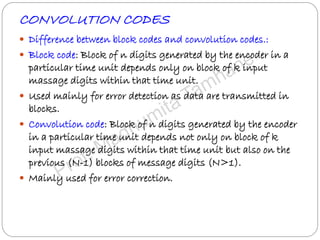
CONVOLUTION CODES
 Difference between block codes and convolution codes.:
 Block code: Block of n digits generated by the encoder in a
particular time unit depends only on block of k input
massage digits within that time unit.
 Used mainly for error detection as data are transmitted in
blocks.
 Convolution code: Block of n digits generated by the encoder
in a particular time unit depends not only on block of k
input massage digits within that time unit but also on the
previous (N-1) blocks of message digits (N>1).
 Mainly used for error correction.

TREE CODES and TRELLIS CODES
• Input stream broken into m segments of ko symbols
each.
• Each segment – Information frame.
• Encoder – (Memory + logic circuit.)
• m memory to store m recent information frames
at a time. Total mko information symbols.
• At each input, logic circuit computes codeword.
• For each information frames (ko symbols), we get a
codeword frame (no symbols ).
• Same information frame may not generate same
code word frame. Why?

TREE CODES
ko ko ko ko ko ko ko
Logic no
Encoder
Constraint Length v = mko
Information Frame
Codeword Frame
•Constraint length of a shift register encoder is
number of symbols it can store in its memory.
• v = mko

TREE CODES – some facts/definitions!
 Wordlength of shift register encoder k = (m+1)ko
 Blocklength of shift register encoder n = (m+1)no
 (no,ko)code tree rate = ko/no =k/n.
 A (no,ko) tree code that is linear, time invariant and
has finite Wordlength k = (m+1)ko is called (n,K)
Convolution codes.
 A (no,ko) tree code that is time invariant and has
finite Wordlength k = (m+1)ko is called (n,K)
Sliding Block codes. Not linear.

Convolution Encoder
• One bit input converts to two bits code.
• ko =1, no= 2, Block length = (m+1)no =6
• Constraint length = 2 , Code rate = ½
+
++
Shift RegisterInput Encoded output

Convolutional Encoder- Input and output bits
Incoming
Bit
Current state of
Encoder
Outgoing Bits
0 0 0 0 0
1 0 0 1 1
0 0 1
1 0 1
0 1 0
1 1 0
0 1 1
1 1 1

Convolutional Encoder- Input and output bits
Incoming
Bit
Current state of
Encoder
Outgoing Bits
0 0 0 0 0
1 0 0 1 1
0 0 1 1 1
1 0 1 0 0
0 1 0 0 1
1 1 0 1 0
0 1 1 1 0
1 1 1 0 1

Convolutional Encoder - State Diagram
 Same bit gets coded differently depending upon
previous bits.
 Make state diagram of Encoder.
 2 bits encoder – 4 states.

Convolutional Encoder - State Diagram
01
10
1100
0
0
0
0
1
1
1
1

Convolutional Encoder - Trellis codes/Diagram
 4 Nodes are 4 States. Code rate is ½.
 In trellis diagram, follow upper or lower branch to
next node if input is 0 or 1.
 Traverse to next state of node with this input,
writing code on the branch.
 Continues…
 Complete the diagram.

Convolutional Encoder - Trellis Diagram
00
10
01
11
00
11
States

Convolutional Encoder - Trellis Diagram
00
10
01
11
00
11
States
00 00 00
11 11
01
10
00
10
01

Trellis Diagram – Input 1 0 0 1 1 0 1
Output – 11 01 11 11 10 10 00
00
10
01
11
00
11
States
00 00
11 11
01
10
00
10
01
00 00 00
11
10
10
00

Convolutional Encoder - Polynomial
description
 Any information sequence i0, i1, i2, i3, …can be
expressed in terms of delay element D as
 I(D) = i0 + i1 D + i2 D2 + i3 D3 + i4D4 + …
 10100011 will be 1+ D2 + D6+ D7

Convolutional Encoder - Polynomial
description
• Similarly, encoder can also be expressed as
polynomial of D.
• Using previous problem, ko =1, no= 2,
– first bit of code g11(D)= D2+D+1
– Second bit of code g12(D)= D2+1
– G(D) = [gij(D)]= [D2+D+1 D2+1]
 cj(D) = ∑i il(D)gl,j(D)
C(D) = I(D)G(D)

Convolutional encoder – Example
Find Generator polynomial matrix, rate of code
and Trellis diagram.
i ab
+

 k0 = 1, n0 = 2, rate = ½.
 G(D) = [1 D4+1]
 Called systematic convolution encoder as k0 bits of
code are same as data.

Find Generator polynomial matrix, rate of code
and Trellis diagram.
k2
k1
n1
n2
n3
++

• k0 = 2, n0 = 3, rate = 2/3.
• G(D) = g11(D) g12(D) g13(D)
• g21(D) g22(D) g23(D)
= 1 0 D3+D+1
0 1 0

Convolutional encoder – Formal definitions
 Wordlength k = k0 maxi,j{deg gij (D) + 1].
 Blocklength n = n0 maxi,j{deg gij (D) + 1].
 Constraint length
v = ∑ maxi,j{deg gij (D)].
 Parity Check matrix H(D) is (n0-k0) by n0 matrix
of polynomials which satisfies-
 G(D) H(D)- 1= 0
 Syndrome polynomial s(D) is (n0-k0) component
row vector
 s(D) = v(D) H(D)- 1

Convolutional encoder – Formal definitions
 Systematic Encoder has G(D) = [I | P(D)]
 Where I is k0 by ko identity matrix and P(D) is ko by (
n0-k0) parity check polynomial given by
 H(D) = [-P(D)T |I]
 Where I is ( n0-k0) by( n0-k0) identity matrix.
 Also G(D) H(D)T = 0

Convolutional encoder – Error correction
 lth minimum distance dl* is smallest hamming
distance between any two initial codeword segments
l frames long that are not identical in initial frames.
 If l=m+1, then (m+1)th minimum distance is
minimum distance of the code d* or dmin..
 Code can correct “t” errors in first l frames if
 dl* ≥ 2t+1

Convolutional encoder -Example
 m = 2, l = 3
 d1*=2, d2*=3, d3*=5… comparing with all ‘0’s.
 d* = 5
 t = 2

Convolutional encoder – Free Distance
 Minimum distance between arbitrarily long encoded
sequence. ( Possibly infinite)
 Free distance is dfree = maxl[dj]
 It can be minimum weight of a path that deviates
from the all zero path and later merges back into the
all zero path.
Also dm+1 ≤ dm+2 ≤ …≤ dfree

Convolutional encoder – Free Length
 Free length nfree is length of non-zero segment of
smallest weight convolution codeword of nonzero
weight.
 dl = dfree if l = nfree.

Convolutional encoder – Free Length
 Here
 Free distance = 5
 Free length = 6
00
10
01
11
00
11
00 00
11 11
01
10
00
10
01
00 00 00
11
10
10
00

Matrix description of Convolution encoder - Example

Matrix description of Convolution encoder -
Example
 Generator polynomials are:
 g11(D) = D + D2
 g12(D) = D2
 g13(D) = D + D2
 g21(D) = D2
 g22(D) = D
 g23(D) = D

Example
 Matrix G0 has coefficients of D0 i.e. constant s:
 Matrix G1 has coefficients of D1 :
 Matrix G2 has coefficients of D2 :

Example
 Generator matrix is only the representation of a
convolution coder. It is actually not used to generate
codes.
1 0 0
1 0 0

Matrix description of Convolutional encoder - General
 Generator matrix is only the representation of a
convolution coder. It is actually not used to generate
codes.

VITERBI DECODING
 Advantages:
 Highly satisfactory bit error performance
 High speed of operation.
 Ease of implementation.
 Low cost.

VITERBI DECODING
• Given Trellis Diagram of rate 1/3.
• Transmitted word – 000000000000000000000…
• Received word – 010000100001…

VITERBI DECODING
 Procedure:
 Divide the incoming stream into groups of three.
 010 000 100 001…
 Find hamming distances between first group with two
options at first node. Called Branch Metric.
 Take second group and continue with second node.
Find total hamming distance called Path Metric.
 At any node if two branches meet, discard branch
with higher Path Metric.
 Continue…

VITERBI DECODING
• First group - 010
• d(000,010) = 1 BM1 = 1
• d(111,010) = 2 BM2 = 2

VITERBI DECODING
• Second group – 000
• Branch Metric and Path Metric(circled) are found.
• At each node three compare total path metric.

VITERBI DECODING
• Third group – 100
• At each node three compare total path metric.
• Discard longer Path and retain Survivor.

VITERBI DECODING
• Continue…

Assignments:
 1. Design a rate ½ Convolutional encoder with a
constraint length v = 4 and d* = 6.
 Construct state diagram for this encoder.
 Construct trellis diagram.
 What is dfree for this code.
 Give generator matrix G.

• 2 ) For given encoders each, construct Trellis
Diagram. Find k0, n0, v, m, d* and dfree. Find G.

• 3) Write k, n, v, m and Rate R for this coder.
• Give Generator polynomial matrix G(D), generator matrix G
and Parity check matrix H.
• Find d*, dfree, nfree.
• Encode 101 001 001 010 000

CONVOLUTION CODES – using Code Tree
 M1, M2, M3, M4 are 1 bit storage elements feeding
to 3 summers as per design of the code.
 v1, v2, v3 are commutator pins, to be sampled one
after the other.
M1 M2 M4
I/P data stream b1
MSB in first
M3
v1
v2
v3
Code output bo
Commutator

 v1 = s1.
 v2 = s1 ⊕ s2 ⊕ s3 ⊕ s4
 v3 = s1 ⊕ s3 ⊕ s4
 I/p stream enters registers one by one with MSB going in
first.
 As each bit enters, logic summer gives 3-bit O/p v1v2v3.
 Enough zeroes to be added so that last bit leaves m4.
M1 M2 M4
I/P data stream b1
MSB in first
M3
v1
v2
v3
Code output bo
Commutator

 Code generated by combining outputs of m stage
shift registers, through n EX-OR’s .
 No of bits in message stream = L.
 No of bits in output code = n (L + m).
M1 M2 M4
I/P data stream b1
MSB in first
M3
v1
v2
v3
Code output bo
Commutator

 Input stream m=1 0 1 1 0
 L = 5, n = 3, m = 4
 Code bits = 27
 Rate of code = 1/3
 CODE bo = 111 010 100 110 001 000
011 000 000
M1 M2 M4
I/P data stream b1
MSB in first
M3
v1
v2
v3
Code output bo
Commutator

 Code depends on
 No of shift registers m.
 No of shift summers n.
 No of shift input bits L.
 Manner in which all are connected.
M1 M2 M4
I/P data stream b1
MSB in first
M3
v1
v2
v3
Code output bo
Commutator

Code Tree
• Code words = 2kL where –
– L = length of information sequence
– k = number of bits at each each clock
• L+m+1 tree levels are labeled from 0 to L+m.
• The leftmost node A in the tree is called the origin node.
• 2k branches leaving each node in first L levels for an
(n,k,m) code – called Dividing part of the tree.
• Upper branch leaving each node in dividing part of tree
represent input ui =0/1 while lower branch represent
input ui= 1/0.
• After L time units, there is only one branch leaving
each node.
• This represents input 0 for i= L, L+1, …L+m-1 with
encoder returning to all zero state.(Tail of tree)

Code Tree
 2kL Rightmost nodes are called terminal nodes.
 Each branch is labeled with n outputs .
 Each of 2kLcodewords of length N is represented by
a totally distinct path through the tree.
 Code tree contains same information about code as
the trellis diagram or state diagram.
 Tree better suited for operation of sequential
decoding.

Code Tree
0
1
000
111
A
BB
B
C
C
C
C
000
000
010
101
010
111

Decoding the convolution code
 EXHUSTIVE SEARCH METHOD : With no noise
 Start at A.
 Take first n-bit s and compare with two sets of n-
bits connected to A.
 If input matches with a n-bit set of tree for which we
have to go up the tree, decoded data first bit is “0”.
 If input matches with a n-bit set of tree for which we
have to go down the tree, decoded data first bit is “1”.
 Go to nodes B, C etc and repeat the process to decode
other bits.

• EXHUSTIVE SEARCH METHOD : With noise
• Each input message bit effects m x n bits of the code
• = 4X3 = 12 bits.
• At node A , we must check first 12 bits only.
• 16 such unique 12-bit combinations from A.
• Compare first 12 bits with 12 combinations and
select best match.
• If it takes up the tree at A, first bit decoded to “0”
• If it takes down the tree at A, first bit decoded to “1”.
• Discard first 3 bits of input code and repeat the
same at B comparing next 12 bits with next 16
combinations…..and so on.

 EXHUSTIVE SEARCH METHOD : With noise
 Discard first 3 bits of input code and come to node
B.
 Repeat the same at B comparing next 12 bits with
next 16 combinations…..and so on.
 Disadvantages:
 Although it offers low probability of errors, we have
to search mXn code bits in 2m branches. Lengthy.
 Errors tend to propagate . If incorrect direction is
chosen at a node due to more errors. No coming
back.

Decoding the convolution code-
SEQUENTIAL DECODING METHOD
 Sequential decoding was first introduced by
Wozencraft as first practical decoding method for
convolution code.
 Later Fano introduced new version of sequential
decoding called Fano’s algorithm.
 Then another version called the stack or ZJ
algorithm was discovered independently by
Zigangirov and Jelinek.

Wozencraft SEQUENTIAL DECODING
METHOD : With noise
 n bits at a time are considered at a node.
 At node A. we move in the direction of least
discrepancies and decode accordingly.
 No of discrepancies are noted.
 Move to node B and repeat.
 At every node compare no of discrepancies with
already decided maximum permissible errors.
 If current error exceed decided value at any node,
traverse back one node and take the other direction.
 Repeat the process.

Number of message bits decoded
Total no of
discrepancies at
a node or errors
while decoding
Discard level
(1)
(4)
(3)
(2)
Correct Path

SEQUENTIAL DECODING METHOD
 Advantages:
 Works on smaller code blocks.
 Faster.
 Although trial and error and retracing involved,
still gives better results at smaller time.

ASSIGNMENT find code tree.
M1 M2
3 bit input
M3
v1
v2
v3
Code output bo
Commutator

The Stack Algorithm – ZJ Algorithm
• Let input data stream length is L with k bits
entering simultaneously in each of L.
• Information sequence length = kL
• 2kL code words of length N = n(L+m) for (n.k,m)
code where
– Number of memory element = m
– Number of summer = n
• Code tree has L+m+1 time units or levels.
• Code tree is just expanded version of trellis diagram
in which every path is totally distinct from every
other path.
• Method searches through the nodes of tree to find
maximum likelihood path by measuring “closeness”
called metric.

 Example: (3,1,2) convolution coder has generator
matrix as
 G(D) = [1+D, 1+D2, 1+D+D2]
 Let L=5. n=3, k=1, m=2
 L+m+1=8 tree levels from 0 to 7.
 The code tree is-

 For binary input and Q-ary output DMC, bit metric -
 M(ri|vi) = log2[P(ri|vi) / P(ri)] – R
 Where P(ri|vi) is channel transition probability,
 P(ri) is channel output symbol probability,
 R is code rate.
 The above includes length of path in metric.
 Partial path metric for first l branches of a path v –
 M([ri|vi]l-1) = ∑j=0
l-1
M(rj|vj) = ∑i=0
nl-1
M(ri|vi)
 Where M(rj|vj) is branch metric of jth branch and is
computed by adding bit metric for the n bits on that
branch.
 Combining above two-

 M([ri|vi]l-1) =
 ∑i=0
nl-1
log2P(ri|vi) - ∑i=0
nl-1
P(ri) – ∑i=0
nl-1
R
 A binary input Q-ary out put DMC is said to be
symmetric if –
 P(j|0) = P(Q-1-j|1), j=0,1,2…Q-1
 e.g. Q=2, P(j|0) = P(1-j|1),
 For symmetric channel with equally likely i/p symbols,
o/p symbols are also equally likely. Then-
 P(ri=j) = 1/Q , 0≤j≤Q-1 e.g. Q=2, P(0)=P(1)=1/2.
 M([ri|vi]l-1) = ∑i=0
nl-1
log2P(ri|vi) – nl log2(1/Q)– nlR
 = ∑i=0
nl-1
log2P(ri|vi) + nl(log2Q – R)

 M([ri|vi]l-1)= ∑i=0
nl-1
log2P(ri|vi) + nl(log2Q – R)
 First term is metric for Viterbi algorithm.
 Second term represents a positive bias (Q≥2, R≤1), which
increases linearly with path length.
 Hence longer paths with larger bias are closer to ‘End of
tree” and more likely to be Maximum Likelihood path.
 Called Fano Metric as first introduced by Fano.

 Example: For BSC(Q=2) with transition probability p,
find Fano metric for truncated codeword [v]5 and [v’]0.
Also find metric if p=0.1.
 [v]5 is shown in code tree by thick line. 2 bits in error out
of 18.
 M([r|v]5)= 16log2(1-p) + 2log2p + 18( 1-1/3 )
 = 16log2(1-p) + 2log2p + 12
 M([r|v’]0)= 2log2(1-p) + log2p + 3( 1-1/3 )
 = 2log2(1-p) + log2p + 2
 If p=0.1,
 M([r|v]5)= 2.92 > M([r|v’]0)= -1.63

 For BSC with transition probability p, the bit metrics are
 M(ri|vi) = log2[P(ri|vi) / P(ri)] – R
 = log2 P(ri|vi) - log2P(ri) – R
 P(ri) = ½.
 M(ri|vi) = log2 p- log2 2 – R
 M(ri|vi) = {log2 2p - R if ri≠ vi
 = log2 2(1-p) – R if ri= vi }

• Example : If R = 1/3 and p = 0.10, find M(ri|vi)
• M(ri|vi) = {-2.65 if ri≠ vi
• = 0.52 if ri= vi }
• The metric table is shown below.
• Metric table is usually scaled by positive constant to
approximate values to integers. Scaled table is -

Stack Algorithm – ZJ Algorithm - Method
 An ordered list or stack of previously examined paths of
different lengths is kept in storage.
 Each stack entry contains a path along with its metric.
 Path are listed in stack in order of decreasing metric.
 At each decoding step, top path of stack is extended by
computing the branch metrics of its 2k succeeding
branches and adding these to metric of top path to form 2k
new paths, called successors of the top path.
 Top path is then deleted from the stack, its 2k successors
are inserted and stack is rearranged in decreasing order
of metric values.
 Algorithm terminates when top path is at the end of tree.

The Stack Algorithm
 Step 1 : Load the stack with the origin node in the tree,
whose metric is taken to be zero.
 Step 2: Compute the metric of the successor of the top path
in the stack.
 Step 3: Delete the top path from the stack.
 Step 4: Insert the new paths in the stack and rearrange
the stack in order of decreasing metric values.
 Step 5: If the top path in the stack ends at a terminal node
in the tree, stop. Otherwise returning to step 2.
 When the algorithm terminates, the top path in the stack
is taken as decoded path.
 Make flowchart for the stack algorithm.

The Stack -more facts
 In the dividing part of the tree , there are 2k new metrics to
be computed at step 1.
 In the tail of the tree, only one new metric is computed.
 For (n,1,m) codes, size of stack increases by one for each
decoding step except at tail of tree, where size of stack does
not increase at all.
 Since dividing part of tree is much longer than tail
(L>>m), the size of stack is roughly equal to the number
of decoding steps when algorithm terminates.

The Stack Algorithm -Example
• Consider the earlier R=1/3 code tree and apply stack
algorithm. Assume a code word is transmitted over a BSC
with p=0.10 and the following sequence is received. Using
metric table, show content of stack stepwise and decode
correct word.
• r = (010, 010, 001, 110, 100, 101, 011
• Take first n=3 bits at first dividing part and compare
with two branches to find toe branch matrics.
• 010 with 111 at upper branch (1) gives 2 discrepancies
and 1 match.
• From table branch metric = 2X (-5) + 1X1 = -9
• 010 with 000 at lower branch (0) gives 1 discrepancy and
2 match.
• From table branch metric = 1X (-5) + 2X1 = -3

-Example
• Step 1 path and path metric arranged in decreasing order in
stack above.
• Top path is extended to two parts and 2nd set 010 is compared
with 111(1) and 000(0). Branch metric added to previous path
metric.
• Upper branch – 1 match and 2 discrepancy.
• Path metric = -3 + (1X1 + 2X(-5)) = -12 path(01)
• lower branch – 2 match and 1 discrepancy.
• Path metric = -3 + (2X1 + 1X(-5)) = -6 path(00)
• Table modified with new path metric in decreasing order.
• Procedure continues.

The Stack Algorithm -Example
 The algorithm terminates after 10 decoding steps giving
final decoding path and information sequence as –
 C= (111, 010, 001, 110, 100, 101, 011)
 u = (11101)
 Ties in the metric values are resolved by placing the
longest path on top.
 This sometimes, has the effect of slightly reducing the
total number of decoding steps.

The Stack Algorithm –Example -2
 Let received code is r=(110, 110, 110, 111, 010, 101, 101)
 Solution: This sequence terminates after 20 steps and
gives—
 C = (111, 010, 110, 011, 111, 101, 011)
 u= (11001)

The Stack Algorithm Vs Viterbi Algorithm
 A decoding step for the Viterbi algorithm is the “compare
and select operation” performed for each state in the trellis
diagram beyond time unit m.
 It requires 15 computations to decode the required
sequence in example 1 as compared to only 10
computations in Stack algorithm.
 This advantage of Stack algorithm over Viterbi, is more
prominent when fraction of error is not too greater than
channel transition probability.
 2 out of 21 bits are in error. 2/21 =0.095 ≈ p=0.10.
 If sequence is too noisy, stack algorithm requires too
many computations as compared to again 15 of Viterbi.

The Stack Algorithm Vs Viterbi Algorithm
 Most important difference between sequential decoding
and Viterbi decoding is that the number of computations
performed by a sequential decoder is a random variable
while computational load of the Viterbi algorithm is fixed.
 Very noisy sequence may requires larger number of
computations in Stack algorithm as compared to Viterbi.
 As very noisy sequences occur very rarely, average
number of computations performed by a sequential
decoder is normally much less than fixed number
performed by Viterbi algorithm.

The Stack Algorithm- Limitations
• Limitation 1:
• Decoder tree traces random path back and forth through
the code tree, jumping from node to node.
• Hence Decoder must have an input buffer to store
incoming blocks of sequence waiting to be processed.
• Speed factor of decoder is ratio of computation speed to
speed of incoming data in branches received per second.
• Depending on speed factor of decoder, long searches can
cause input buffer to overflow resulting in loss of data or
Erasure.
• Buffer accepts data at fixed rate of 1/(nT) branches per
second where T is the time interval allotted for each bit.
• Erasure probabilities of 10-3 are common in sequential
decoding.

• Average number of computations and erasure probability
are independent of encoder memory ak.
• Hence codes with large K and large free distance may
result in undetected errors being extremely unlikely.
• Major limitation then is Erasures due to buffer overflow.
• Can be actually beneficial!!
• Erasures usually occur when received sequence is very
noisy.
• It is more desirable to erase such frame than decode it
incorrectly.
• Viterbi will always decode- may result in high errors.
• Seq. Dec. -ARQ system can help in retransmission of
erased frames. (Advantage)

 Limitation 2: Size of stack is finite.
 Stack may fill up before decoding is complete.
 Remedy: Typical stack size is 1000 entries.
 The path at the bottom of stack is pushed out of stack at
next entry.
 The probability that a path on the bottom of the stack
would ever recover to reach the top of the stack and be
extended is so small that the loss in performance is
negligible.

• Limitation 3: reordering stack after each decoding step.
• This can become time very consuming as no of entries
increase.
• Severely limit decoding speed.
• Remedy: Stack –bucket algorithm by Jelinek.
• Contents of stack are not reordered after each step.
• Range of possible metric values is quantized into a fixed
number of intervals.
• Each metric interval is assigned a certain number of
locations in storage , called a bucket.
• When a path is extended, it is deleted from storage and
each new path is inserted as the top entry in the bucket
which includes its metric value.

• No reordering of paths within bucket is required.
• The top path in the top nonempty bucket is chosen to be
extended.
• A computation now involves only finding the correct
bucket in which to place each new path.
• Which is independent of previously extended path.
• Faster than reordering an increasingly larger stack.
• Disadvantage: it is not always the best path that gets
extended but only a very good path. i.e. a path in the top
nonempty bucket or the best bucket.
• Typically if bucket quantization is not too large and
received sequence is not too noisy, best bucket contains the
best path.
• Degradation from original algorithm is very slight. Fast.

The FANO Algorithm
• Sacrifices speed w.r.t.stack algorithm but no storage
required.
• Requires more time as it extends more nodes than stack .
• But stack reordering absent, hence saves time.
• Decoder examines a sequence of nodes in the tree from
origin node to terminal nodes.
• Decoder never jumps from node to node as in stack al..
• Decoder always moves to an adjacent node-
– Either forward – to one of 2k nodes leaving present node,
– Or backward to the node leading to present node.
• Metric of the next node to be examined can be computed by
adding (or subtracting) metric of connecting branch to
metric of present node.

The FANO Algorithm
 This eliminates the need for storing the metrics of
previously examined nodes as done in stack algorithm.
 But some nodes are visited more than once, asking for re-
computation of their metric values.

The FANO Algorithm –Method
• The decoder will move forward through the tree as long as
the examined metric value continues to increase.
• When metric value dips below a threshold, the decoder
backs up and begins to examine other path.
• If no path can be found with metric value above threshold,
the threshold is lowered and decoder attempts to move
forward again with a lower threshold.
• Each time a given node is visited in the forward direction,
the threshold is lower than on the previous visit to that
node.
• This prevents looping in the algorithm.
• The decoder eventually reaches end of tree, terminating
algorithm.

The FANO Algorithm –Detailed Method
• Decoder starts at origin node with the threshold T=0 and
the metric value M=0.
• It looks forward to search best of 2k succeeding nodes, the
one with the largest metric.
• If metric of forward node MF ≥ T, the decoder moves to this
node.
• If END not reached and this node has been examined for
the first time, then “threshold tightening” is performed
– Increase T by the largest possible multiple of a threshold
increment ∆, till it remains below current metric.
• If this node is traversed before, no threshold tightening is
performed.
• Decoder again looks forward to best succeeding node.

 If MF < T, the decoder then looks backward to the
preceding node.
 If metric of backward node being examined ,MB < T,
(B0th <T), T is lowered by ∆ and look forward for best
node is repeated.
 If MF < T and MB ≥ T, decoder moves back to preceding
node, say P.
 If this backward path was already from worst of 2k nodes
succeeding node P, decoder again looks back to node preceding
node P.
 If not, decoder again looks forward to the next best of 2k nodes
succeeding node P and checks if MF ≥ T.

 If decoder looks backward from origin node, preceding
node is assumed to be -∞ and threshold is always lowered
by ∆.
 Ties in metric values can be resolved arbitrarily without
affecting average decoder performance.

The FANO
Algorithm –
Flow Chart

The FANO Algorithm –Flow Chart
Origin – T=0, M=0, MB=-∞
Largest MF ≥ T
Decoder moves to forward node.
If first time, T increased till <T.
Otherwise no change in T
MF <T Looks backward
MF <T
MB <T
T = T - ∆
Looks forward
MF <T
MB ≥T
Moves to
backward node.
If current is worst path,
looks backward
Looks forward

The FANO Algorithm –Example -No Error.
 Let C= 111 010 001 110 100 101 011
 Let ∆ = 1
 Data = 1110100
Step Look MF MB Node Metric T
0 - X 0 0
1 LFB +3 - 1 +3 +3
2 LFB +6 - 11 +6 +6
3 LFB +9 - 111 +9 +9
4 LFB +12 - 1110 +12 +12
5 LFB +15 - 11101 +15 +15
6 LFB +18 - 111010 +18 +18
7 LFB +21 - 1110100 +21 Stop
LFB - Look forward to best node LFNB - Look forward to next best node

The FANO Algorithm –Example -With Error.
 Let V= 010 010 001 110 100 101 011. Let ∆ = 1

The FANO Algorithm –Example -With Error.
 Let V= 010 010 001 110 100 101 011. Put∆ = 3

The FANO Algorithm –Limitations
 Number of computations depends upon threshold
increment ∆.
 If ∆ is too small, large number of computations required.
 ∆ can not be raised indefinitely without affecting error
probability.
 If ∆ is too large, T may be lowered below the minimum
metric of the maximum likelihood path along with several
other paths, making it possible for any of these to be
decoded before maximum likelihood path.
 In addition, number of computations also increase as
more “bad” paths can be followed if T is lowered too much.

The FANO Algorithm –Limitations
 For moderate rates, Fano algorithm is faster than stack
bucket algorithm as it is free from stack control problems.
 For higher rates, stack bucket algorithm can be faster as
Fano algorithm would have additional computational
loads .
 As it does not require storage Fano algorithm is selected
in practical implementations of sequential decoding..

Convolution codes - Coding/Decoding Tree codes and Trellis codes for multiple error correction

Recommandé

Recommandé

Contenu connexe

Tendances

Tendances (20)

En vedette

En vedette (8)

Similaire à Convolution codes - Coding/Decoding Tree codes and Trellis codes for multiple error correction

Similaire à Convolution codes - Coding/Decoding Tree codes and Trellis codes for multiple error correction (20)

Plus de Madhumita Tamhane

Plus de Madhumita Tamhane (20)

Dernier

Dernier (20)

Convolution codes - Coding/Decoding Tree codes and Trellis codes for multiple error correction