j

1. Topic 1: Introduction to Probability
Maleakhi Agung Wijaya
Contents
1 Random Experiment 3
1.1 Sample Spaces . . . . . . . . . . . . . . . . . . . . . . . . . . . . . . . . . . . 3
1.2 Events . . . . . . . . . . . . . . . . . . . . . . . . . . . . . . . . . . . . . . . . 3
1.3 Set Operations . . . . . . . . . . . . . . . . . . . . . . . . . . . . . . . . . . . 4
2 Probability 5
3 Conditional Probability 6
3.1 Definition . . . . . . . . . . . . . . . . . . . . . . . . . . . . . . . . . . . . . . 6
3.2 Independence of Events . . . . . . . . . . . . . . . . . . . . . . . . . . . . . . 6
4 Bayes Theorem 8
4.1 Law of Total Probability . . . . . . . . . . . . . . . . . . . . . . . . . . . . . . 8
4.2 Bayes Formula . . . . . . . . . . . . . . . . . . . . . . . . . . . . . . . . . . . 8
Introduction
Welcome to the first topic in my Probability course! Before we start our journey, I want to
talk about the importance of learning probability. Probability is widely used in numerous
career fields, such as Data Science, Mathematics, Actuarial, Finance & Economics, and
many more. Probability is also significantly used in our daily life for making decision. By
learning probability, you would be able to make a more mathematically sound decision.
Let’s have a look at these 2 common situation in which we can find in our daily life.
Monty Hall Problem
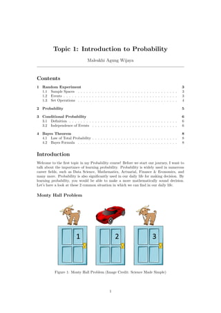
Figure 1: Monty Hall Problem (Image Credit: Science Made Simple)
1

2. CONTENTS CONTENTS
Question: Imagine that you are a contestant of a game show. A prize (car) lies behind
one of three doors. You are asked to chooses a door. Afterward, the host of the show (who
knows which door the prize is behind) opens a door in which the contestant not choose and
which does not have the prize behind it. The host then offers you to either change to the
other unopened door or stick with the original selection. What will you do?
Answer: The formal solution of this problem can be answered using concept from Condi-
tional Probability. However, let’s try to solve this using intuition. When we are asked to
choose the first time, the probability of getting goat is 2
3 , while the probability of getting
car is 1
3 . Then, the host will open the door which does not contain the car and the door
in which we have chosen. During this step, the host effectively eliminate 1 empty door and
this resulted in 2 remaining doors (our chosen door, and another door). Therefore, if we
employ the switch strategy, we will have 2
3 probability of winning the car while if we stick
to the original door, our probability of winning is only 1
3 since it will be more likely that we
will get empty door during the first round of choosing. Therefore, the rational strategy to
maximize the probability of winning is to always switch.
Birthday Problem
Question: You are in a classroom with 9 other students. What is the probability that there
are at least two people present having the same birthday date?
Answer: We can first compute the probability that no person share the same birthday
date. It can be computed by noticing that the first person can choose 365 days for his/her
birthday, second person can choose 364 days since the first person have chosen, third person
can choose 363 days, and so on. Afterward, we take the tail/ complement probability to get
the probability required by the question. Assume that number of days in a year is consistent
365 days.
P(no person share the same date) =
365
365
×
364
365
· · · ×
356
365
= 0.8831
Now, taking the tail probability, we have that
P(at least two people share the same date) = 1 − 0.8831
= 0.1169
Hopefully, you are convinced that probability is really useful for our daily life. Without
further ado, let’s begin our first section about Random Experiment.
Maleakhi Agung Wijaya Page 2

3. 1 RANDOM EXPERIMENT
1 Random Experiment
Random Experiment is a real-life phenomena that is random/ non-deterministic, can be
repeated, and relative frequency stabilize around some value as the number of experiment
increases. Random Experiment produces numerous possible outcomes in which can be cap-
tured using set notations that are described below.
1.1 Sample Spaces
Sample space (Ω) is a set which contains all possible outcomes. The element of this set is
an outcome (ω). The subset of omega in which we can defined probability is universally
called events A. Note that not every subset of omega can be assigned probability. There
are some subset of omega in the general case in which we cannot assign probability.
Example:
1. Tossing coin until the first head shows up
Sample space: {H, TH, TTH, TTTH, TTTTH, ...}
2. Tossing ordinary dice once
Sample space: {1, 2, 3, 4, 5, 6}
3. Tossing two ordinary coins
Sample space: {HH, TH, HT, TT}
1.2 Events
Events are subsets of Ω in which probability can be assigned. If the sample spaces Ω has
countable outcomes, then all subsets can be assigned probability. However, if it is countable
then there are no guarantee that we can assigned probability to all subsets of Ω. For exam-
ple, choosing a number out of Real Number line cannot be assigned a probability.
Example: we would like to model events and outcome space using set notations based on
knowledge that we have gained.
Consider choosing a student from a lecture theatre. We want to represent events that
the student:
1. is NOT playing sport regularly;
2. was born in UK OR Australia;
3. is a male AND less than 20 y.o.
Expressing what we wanted, consider the following using set operations:
1. Let Ω := population of all students in the lecture theatre, A := sub-population of stu-
dents who play sport regularly. Therefore, we can take the complement and represent
using Ac
:= {ω ∈ Ω : ω ∈ A}.
2. Consider B := students born in UK, C := students born in Australia. Therefore, the
B ∪ C := {ω ∈ Ω : ω ∈ B ∨ ω ∈ C}.
3. Consider D := sub-population of male students, E := sub-population of students < 20
years. Similarly, it can be represented using D ∩ E := {ω ∈ Ω : ω ∈ D ∧ ω ∈ E}.
Maleakhi Agung Wijaya Page 3

4. 1.3 Set Operations 1 RANDOM EXPERIMENT
1.3 Set Operations
It is crucial to be able to manipulate set as events are naturally define using sets. Listed
below is a common way to define events using set notations.
• The event A ∪ B is the event that A or B or both occurs.
• The event A ∩ B is the event that A and B both occurs.
• The event Ac
is the event that A does not occur.
• Two events A1 and A2 are disjoint if A1 ∩ A2 = ∅.
• Events A1, A2, A3, ... is called exhaustive if
∞
i=1
Ai = Ω.
• If Ai is disjoint and exhaustive, then we called it a partition.
Hint: It is recommended to draw Venn Diagram to model problem related to sets
Maleakhi Agung Wijaya Page 4

5. 2 PROBABILITY
2 Probability
Earlier we mention that we want to assign probability to events, but what is probability? I
defined probability as measurement that can be used to quantify the likelihood of an event.
However, it is hard to interpret the meaning of a number attach to the event. Generally,
there are 2 interpretation of probability:
1. Relative Frequency Interpretation
It will be easier to explain this using example. If we attach a fraction such as 1
2 as the
probability of getting odd numbers in a dice roll. Then intuitively we can interpret
this as if we roll the dice n times, then we can expect to have n
2 odd numbers.
2. Bayesian Interpretation
Consider attaching 1
3 as the probability of certain species will extinct. We cannot
interpret this using Relative Frequency as we cannot simulate this event continuously.
Therefore, the number is interpreted as a degree of belief of the person attaching it
to the event where certain species extinct. This is what we usually called Bayesian
Probability.
Mathematician approach the problem of quantifying a probability to events through the use
of axioms. The following is going to be how we will define probability in my course.
Definition: Probability is defined as a set function P : F → R where F is defined as set of
subsets of Ω1
such that:
1. P(A) ≥ 0;
2. P(Ω) = 1;
3. For any pairwise disjoint A1, A2, ...,
∞
i=1
Ai =∞
i=1 Ai.
Based on the axioms, there are some other properties of probability which we can defined
as follow:
1. P(∅) = 0
2. P(Ac
) = 1 − P(A)
3. A ⊂ B ⇒ P(A) < P(B)
4. For any events A and B,
P(B ∪ A) = P(B) + P(A) − P(B ∩ A)
Example: Consider the following example of attaching probability to events using axioms
described above.
• Roll of a dice
P(getting any number) = 1
6
• Getting 2 heads in a row
P(getting 2 heads in a row) = 1
4
1F is defined as a σ − algebra, but don’t worry about this for now
Maleakhi Agung Wijaya Page 5

6. 3 CONDITIONAL PROBABILITY
3 Conditional Probability
3.1 Definition
Conditional probability is defined as a measure of the probability of an event occurring given
that another event has occurred (Wikipedia).
Example: Consider the experiment of rolling 2 dice.
• Let event A be the event that the sum of both rolls are < 6.
• Let event B be the event that we got 3 on the first roll.
• We wish to calculate probability of A occurring given that we know B has occurred.
A notation that can be used is using the ”conditional probability” notation P(A|B).
.
To solve this example, we can list all possibilities and calculate the probability. Consider
all possible scenarios {(3, 1), (3, 2), (3, 3), (3, 4), (3, 5), (3, 6)}. By listing all possibilities we
know that P(A|B) = 2
6 = 1
3 .
We don’t really need to always listing all possibilities in order to calculate conditional prob-
ability. There is a general formula for conditional probability that can be derived easily
using intuition.
Definition: Consider 2 events A an d B with P(B) > 0. The conditional probability of A
given B can be calculated as follow:
P(A|B) =
P(A ∩ B)
P(B)
Intuitively, it can be understood as sample size reduction. Observe the following venn
diagram below. Consider that we have the information that B has occurred, if we want
to calculate the probability of A, then we can just calculate the intersection (A ∩ B) and
compare it with the reduced sample size (B). Try to attempt the question above using both
intuition and formula!
Figure 2: Conditional Probability
3.2 Independence of Events
Consider events A and B, there are 3 possible relationships between A and B.
1. Positive relationship when P(A|B) > P(A). This relationship means that the
likelihood of A appearing will increase given that B occurred.
Maleakhi Agung Wijaya Page 6

7. 3.2 Independence of Events 3 CONDITIONAL PROBABILITY
2. Negative relationship when P(A|B) < P(A). This relationship means that the
likelihood of A appearing will decrease given that B occurred.
3. Independent relationship when P(A|B) = P(A). This relationship means that A
is independent of B which implies that given that we know that B occurred, it won’t
change the likelihood of A occurs.
Definition: Events A1, A2, ... are independent with each other if and only if
P(A1 ∩ A2 ∩ A3 ∩ ...) =
∞
i=1
P(Ai)
Based on the definition, we know that independent is not the same with mutual exclusion
or disjoint. For disjoint, the intersection is empty set, but it is not necessarily the case with
independent events. Back to the definition given above, we can prove using the following
method; we can consider base case of having 2 events and show that this theorem hold. To
finish off, we can then proof the inductive case and conclude using proof by induction which
is left to curious reader.
Proof: If A and B are independent, then P(A ∩ B) = P(A)P(B)
First, consider the definition from Conditional Probability section that P(A|B) = P (A∩B)
P (B) .
Secondly, we also know by independent assumptions that P(A|B) = P(A).
∴ Thus, using substitution and above statements, we have that P(A) = P (A∩B)
P (B) . Rearrang-
ing this equation, we have that P(A ∩ B) = P(A)P(B) as required.
Q.E.D
Corollary: If A1, A2, A3, ..., An are independent events, then any combination of comple-
ments are also independent.
• A1, A2, A3, Ac
4, ..., Ac
n is independent
• Ac
1, A2, A3, Ac
4, ..., Ac
n is independent
• and any other combinations
Example: A student has 0.25 probability of getting right answer in an exam consisting of
8 questions. Assuming independence between questions, what is the probability that the
student getting correct answers for everything except last question?
Solution: Using independent definition, P(getting everything correct except last question) =
0.257
× (1 − 0.25).
Maleakhi Agung Wijaya Page 7

8. 4 BAYES THEOREM
4 Bayes Theorem
4.1 Law of Total Probability
Partition of an event is collection of disjoint and exhaustive 2
events. Consider the figure
below as an example of partition of an event A. In this picture, we can see that event A
is partitioned by A1, A2, A3, A4, A5, A6. To check that this is partition we can simply look
and conclude since all sub-events does not overlap with each other, and
6
i=1
Ai = A.
Figure 3: Partition of event A
Partition is useful as a tools to compute probability. In general case if an event is partition
into several elements, we can calculate the probability of the event by summing all of the
elements From example above, we can compute probability of event A, by summing all of
the partitions, i.e. P(A) = P(A1) + P(A2) + ... + P(A6). This statement holds true due to
disjointness property and exhaustivity of the partition definition. Let’s now use this intu-
ition to derive the Law of Total Probability.
Theorem: Law of Total Probability can be derived as follows. Consider general event A
which is partitioned into A1, A2, A3, ..., An. Using our intuition from partition, we can then
derive the following:
P(A) =
n
i=1
P(Ai)
=
n
i=1
P(A ∩ Ai)
=
n
i=1
P(A|Ai)P(Ai)
The last line of the equation is what we famously known as Law of Total Probability (LOTP)
and is extensive used to calculate probability of a complex events.
4.2 Bayes Formula
Recall the conditional probability formula given in section 3.1. Sometimes it is easier to
modify the formula to include P(B|A)P(A) instead of using P(A ∩ B). The formula is
derived as follows:
2see text 1.3 for definition
Maleakhi Agung Wijaya Page 8

9. 4.2 Bayes Formula 4 BAYES THEOREM
Theorem: To derive Bayes Formula, recall that using Conditional Probability formula, we
can write P(B|A) = P (A∩B)
P (A) . Therefore, we have that P(A∩B) = P(B|A)P(A) by algebra.
Now, using this result, we can derive Bayes Formula:
P(A|B) =
P(A ∩ B)
P(B)
=
P(B|A)P(A)
P(B)
This Bayesian Formula has numerous applications. One of the most fundamental usage is
to move from prior probability to posterior probability that are really used in statistics for
inference. In addition, it is also used in numerous Machine Learning Algorithm such as
variety of Naive Bayes, Neural Network, and so on.
To demonstrate the use of LOTP and Bayes Formula let’s do this 2 examples. This
example can be solved easily using the trick that we have discussed in Section 4.
Example:
• Suppose a test for HIV is 90% effective in the sense that if a person is infected by HIV,
then there is 90% probability that the test they are HIV positive.
• If they are not positive, assume that there is still a 5% probability that the test says
that they are. We wish to calculate probability that the person actually is HIV
positive given that the test says so? (Assume 0.0001 population is infected by
HIV)
Answer First let A be the event that the test says a person is HIV positive, and H
be the event that the person is actually HIV positive. Based on the data, we have that
P(A|H) = 0.9, while P(A|Hc
) = 0.05.
We wish to calculate P(H|A) which is given by the following equation using Bayes Formula.
P(H|A) =
P(A|H)P(H)
P(A)
=
0.9 × 0.0001
P(A)
Now, we can solve probability of event A by using Law of Total Probability by partitioning
Ω into H and Hc
.
P(A) = P(A|H)P(H) + P(A|Hc
)P(Hc
)
= 0.9 × 0.0001 + 0.05 × (1 − 0.0001)
= 0.0501
Back to previous equation, we can solve the probability required as follows
P(H|A) = 0.9 ×
0.0001
0.0501
= 0.0018
∴ Therefore, the probability that the person is actually HIV positive given that the test says
so is 0.0018.
Maleakhi Agung Wijaya Page 9

10. 4.2 Bayes Formula 4 BAYES THEOREM
Example: A factory has 3 machines that make parts.
• Machine A makes 20%, of which 6% are defective.
• Machine B makes 40%, of which 7% are defective.
• Machine C makes 40%, of which 10% are defective.
• What is the probability that a random part is defect?
Answer: Let A, be the production of Machine A, B and C respectively. Let D be the
probability a random part is defect. Based from the question above, we have the following:
• P(A) = 0.2
• P(B) = P(C) = 0.4
• P(D|A) = 0.06
• P(D|B) = 0.07
• P(D|C) = 0.1
Using Law of Total Probability, we can get the following results:
P(D) = P(D|A)P(A) + P(D|B)P(B) + P(D|C)P(C)
= 0.06 × 0.2 + 0.07 × 0.4 + 0.1 × 0.4
= 0.08
∴ Therefore the probability of defective is 8%.
Maleakhi Agung Wijaya Page 10

11. REFERENCES REFERENCES
References
[1] Ghahramani, S. (1996). Fundamentals of Probability: With Stochastic Processes, Third
Edition. Boca Raton, Florida: CRC Press.
Maleakhi Agung Wijaya Page 11